Alchemy is a collection of independent library components that specifically relate to efficient low-level constructs used with embedded and network programming.
The latest version of Embedded Alchemy[^] can be found on GitHub.The most recent entries as well as Alchemy topics to be posted soon:
- Steganography[^]
- Coming Soon: Alchemy: Data View
- Coming Soon: Quad (Copter) of the Damned
My previous two entries have presented a mathematical foundation for the development and presentation of 3D computer graphics. Basic matrix operations were presented, which are used extensively with Linear Algebra. Understanding the mechanics and limitations of matrix multiplication is fundamental to the focus of this essay. This entry demonstrates three ways to manipulate the geometry defined for your scene, and also how to construct the projection transform that provides the three-dimensional effect for the final image.
Transforms
There are three types of transformations that are generally used to manipulate a geometric model, translate, scale, and rotate. Your models and be oriented anywhere in your scene with these operations. Ultimately, a single square matrix is composed to perform an entire sequence of transformations as one matrix multiplication operation. We will get to that in a moment.
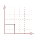
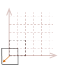
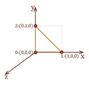
For the illustration of these transforms, we will use the two-dimensional unit-square shown below. However, I will demonstrate the math and algorithms for three dimensions.
| \( \eqalign{ pt_{1} &= (\matrix{0 & 0})\\ pt_{2} &= (\matrix{1 & 0})\\ pt_{3} &= (\matrix{1 & 1})\\ pt_{4} &= (\matrix{0 & 1})\\ }\) |
|
Translate
Translating a point in 3D space is as simple as adding the desired offset for the coordinate of each corresponding axes.
\( V_{translate}=V+D \)
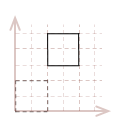
For instance, to move our sample unit cube from the origin by \(x=2\) and \(y=3\), we simply add \(2\) to the x-component for every point in the square, and \(3\) to every y-component.
| \( \eqalign{ pt_{1D} &= pt_1 + [\matrix{2 & 3}] \\ pt_{2D} &= pt_2 + [\matrix{2 & 3}] \\ pt_{3D} &= pt_3 + [\matrix{2 & 3}] \\ pt_{4D} &= pt_4 + [\matrix{2 & 3}] \\ }\) |
|
There is a better way, though.
That will have to wait until after I demonstrate the other two manipulation methods.
Identity Matrix
The first thing that we need to become familiar with is the identity matrix. The identity matrix has ones set along the diagonal with all of the other elements set to zero. Here is the identity matrix for a \(3 \times 3\) matrix.
\( \left\lbrack \matrix{1 & 0 & 0\cr 0 & 1 & 0\cr 0 & 0 & 1} \right\rbrack\)
When any valid input matrix is multiplied with the identity matrix, the result will be the unchanged input matrix. Only square matrices can identity matrices. However, non-square matrices can be used for multiplication with the identity matrix if they have compatible dimensions.
For example:
\( \left\lbrack \matrix{a & b & c \\ d & e & f \\ g & h & i} \right\rbrack \left\lbrack \matrix{1 & 0 & 0\cr 0 & 1 & 0\cr 0 & 0 & 1} \right\rbrack = \left\lbrack \matrix{a & b & c \\ d & e & f \\ g & h & i} \right\rbrack \)
\( \left\lbrack \matrix{7 & 6 & 5} \right\rbrack \left\lbrack \matrix{1 & 0 & 0\cr 0 & 1 & 0\cr 0 & 0 & 1} \right\rbrack = \left\lbrack \matrix{7 & 6 & 5} \right\rbrack \)
\( \left\lbrack \matrix{1 & 0 & 0\cr 0 & 1 & 0\cr 0 & 0 & 1} \right\rbrack \left\lbrack \matrix{7 \\ 6 \\ 5} \right\rbrack = \left\lbrack \matrix{7 \\ 6 \\ 5} \right\rbrack \)
We will use the identity matrix as the basis of our transformations.
Scale
It is possible to independently scale geometry along each of the standard axes. We first start with a \(2 \times 2\) identity matrix for our two-dimensional unit square:
\( \left\lbrack \matrix{1 & 0 \\ 0 & 1} \right\rbrack\)
As we demonstrated with the identity matrix, if we multiply any valid input matrix with the identity matrix, the output will be the same as the input matrix. This is similar to multiplying by \(1\) with scalar numbers.
\( V_{scale}=VS \)
Based upon the rules for matrix multiplication, notice how there is a one-to-one correspondence between each row/column in the identity matrix and for each component in our point..
\(\ \matrix{\phantom{x} & \matrix{x & y} \\ \phantom{x} & \phantom{x} \\ \matrix{x \\ y} & \left\lbrack \matrix{1 & 0 \\ 0 & 1} \right\rbrack } \)
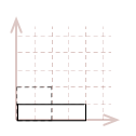
We can create a linear transformation to scale point, by simply multiplying the \(1\) in the identity matrix, with the desired scale factor for each standard axis. For example, let's make our unit-square twice as large along the \(x-axis\) and half as large along the \(y-axis\):
\(\ S= \left\lbrack \matrix{2 & 0 \\ 0 & 0.5} \right\rbrack \)
This is the result, after we multiply each point in our square with this transformation matrix; I have also broken out the mathematic calculations for one of the points, \(pt_3(1, 1)\):
| \( \eqalign{ pt_{3}S &= \\ &= [\matrix{1 & 1}] \left\lbrack\matrix{2 & 0 \\ 0 & 0.5} \right\rbrack\\ &= [\matrix{(1 \cdot 2 + 1 \cdot 0) & (1 \cdot 0 + 1 \cdot 0.5)}] \\ &= [\matrix{2 & 0.5}] }\) |
|
Here is the scale transformation matrix for three dimensions:
\(S = \left\lbrack \matrix{S_x & 0 & 0 \\ 0 & S_y & 0 \\ 0 & 0 & S_z }\right\rbrack\)
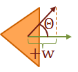
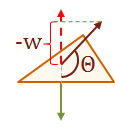
Rotate
A rotation transformation can be created similarly to how we created a transformation for scale. However, this transformation is more complicated than the previous one. I am only going to present the formula, I am not going to explain the details of how it works. The matrix below will perform a counter-clockwise rotation about a pivot-point that is placed at the origin:
\(\ R= \left\lbrack \matrix{\phantom{-} \cos \Theta & \sin \Theta \\ -\sin \Theta & \cos \Theta} \right\rbrack \)
\(V'=VR\)
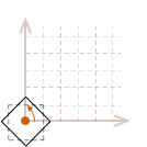
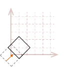
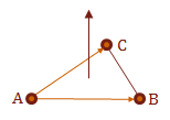
As I mentioned, the rotation transformation pivots the point about the origin. Therefore, if we attempt to rotate our unit square, the result will look like this:
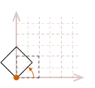
The effects become even more dramatic if the object is not located at the origin:
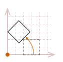
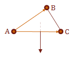
In most cases, this may not be what we would like to have happen. A simpler way to reason about rotation is to place the pivot point in the center of the object, so it appears to rotate in place.
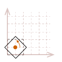
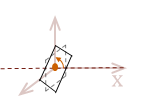
To rotate an object in place, we will need to first translate the object so the desired pivot point of the rotation is located at the origin, rotate the object, then undo the original translation to move it back to its original position.
While all of those steps must be taken in order to rotate an object about its center, there is a way to combine those three steps to create a single matrix. Then only one matrix multiplication operation will need to be performed on each point in our object. Before we get to that, let me show you how we can expand this rotation into three dimensions.
Imagine that our flat unit-square object existed in three dimensions. It is still defined to exist on the \(xy\) plane, but it has a third component added to each of its points to mark its location along the \(z-axis\). We simply need to adjust the definition of our points like this:
| \( \eqalign{ pt_{1} &= (\matrix{0 & 0 & 0})\\ pt_{2} &= (\matrix{1 & 0 & 0})\\ pt_{3} &= (\matrix{1 & 1 & 0})\\ pt_{4} &= (\matrix{0 & 1 & 0})\\ }\) |
|
So, you would be correct to surmise that in order to perform this same \(xy\) rotation about the \(z-axis\) in three dimensions, we simply need to begin with a \(3 \times 3\) identity matrix before we add the \(xy\) rotation.
| \( R_z = \left\lbrack \matrix{ \phantom{-}\cos \Theta & \sin \Theta & 0 \\ -\sin \Theta & \cos \Theta & 0 \\ 0 & 0 & 1 } \right\rbrack \) |
|
We can also adjust the rotation matrix to perform a rotation about the \(x\) and \(y\) axis, respectively:
| R_x = \( \left\lbrack \matrix{ 1 & 0 & 0 \\ 0 & \phantom{-}\cos \Theta & \sin \Theta \\ 0 & -\sin \Theta & \cos \Theta } \right\rbrack \) |
|
| \( R_y = \left\lbrack \matrix{ \cos \Theta & 0 & -\sin \Theta\\ 0 & 1 & 0 \\ \sin \Theta & 0 & \phantom{-}\cos \Theta } \right\rbrack \) |
|
Composite Transform Matrices
I mentioned that it is possible to combine a sequence of matrix transforms into a single matrix. This is highly desirable, considering that every point in an object model needs to be multiplied by the transform. What I demonstrated up to this point is how to individually create each of the transform types, translate, scale and rotate. Technically, the translate operation, \(V'=V+D\) is not a linear transformation because it is not composed within a matrix. Before we can continue, we must find a way to turn the translation operation from a matrix add to a matrix multiplication.
It turns out that we can create a translation operation that is a linear transformation by adding another row to our transformation matrix. However, a transformation matrix must be square because it starts with the identity matrix. So we must also add another column, which means we now have a \(4 \times 4\) matrix:
\(T = \left\lbrack \matrix{1 & 0 & 0 & 0\\ 0 & 1 & 0 & 0\\ 0 & 0 & 1 & 0\\ t_x & t_y & t_z & 1 }\right\rbrack\)
A general transformation matrix is in the form:
\( \left\lbrack \matrix{ a_{11} & a_{12} & a_{13} & 0\\ a_{21} & a_{22} & a_{23} & 0\\ a_{31} & a_{32} & a_{33} & 0\\ t_x & t_y & t_z & 1 }\right\rbrack\)
Where \(t_x\),\(t_y\) and \(t_z\) are the final translation offsets, and the sub-matrix \(a\) is a combination of the scale and rotate operations.
However, this matrix is not compatible with our existing point definitions because they only have three components.
Homogenous Coordinates
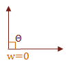
The final piece that we need to finalize our geometry representation and coordinate management logic is called Homogenous Coordinates. What this basically means, is that we will add one more parameter to our vector definition. We refer to this fourth component as, \(w\), and we initially set it to \(1\).
\(V(x,y,z,w) = [\matrix{x & y & z & 1}]\)
Our vector is only valid when \(w=1\). After we transform a vector, \(w\) has often changed to some other scale factor. Therefore, we must rescale our vector back to its original basis by dividing each component by \(w\). The equations below show the three-dimensional Cartesian coordinate representation of a vector, where \(w \ne 0\).
\( \eqalign{ x&= X/w \\ y&= Y/w \\ z&= Z/w }\)
Creating a Composite Transform Matrix
We now possess all of the knowledge required to compose a linear transformation sequence that is stored in a single, compact transformation matrix. So let's create the rotation sequence that we discussed earlier. We will a compose a transform that translates an object to the origin, rotates about the \(z-axis\) then translates the object back to its original position.
Each individual transform matrix is shown below in the order that it must be multiplied into the final transform.
\( T_c R_z T_o = \left\lbrack \matrix{ 1 & 0 & 0 & 0 \\ 0 & 1 & 0 & 0 \\ 0 & 0 & 1 & 0 \\ -t_x & -t_y & -t_z & 1 \\ } \right\rbrack \left\lbrack \matrix{ \phantom{-}\cos \Theta & \sin \Theta & 0 & 0 \\ -\sin \Theta & \cos \Theta & 0 & 0 \\ 0 & 0 & 1 & 0 \\ 0 & 0 & 0 & 1 \\ } \right\rbrack \left\lbrack \matrix{ 1 & 0 & 0 & 0 \\ 0 & 1 & 0 & 0 \\ 0 & 0 & 1 & 0 \\ t_x & t_y & t_z & 1 \\ } \right\rbrack \)
Here, values are selected and the result matrix is calculated:
\(t_x = 0.5, t_y = 0.5, t_z = 0.5, \Theta = 45°\)
\( \eqalign{ T_c R_z T_o &= \left\lbrack \matrix{ 1 & 0 & 0 & 0 \\ 0 & 1 & 0 & 0 \\ 0 & 0 & 1 & 0 \\ -0.5 & -0.5 & -0.5 & 1 \\ } \right\rbrack \left\lbrack \matrix{ 0.707 & 0.707 & 0 & 0 \\ -0.707 & 0.707 & 0 & 0 \\ 0 & 0 & 1 & 0 \\ 0 & 0 & 0 & 1 \\ } \right\rbrack \left\lbrack \matrix{ 1 & 0 & 0 & 0 \\ 0 & 1 & 0 & 0 \\ 0 & 0 & 1 & 0 \\ 0.5 & 0.5 & 0.5 & 1 \\ } \right\rbrack \\ \\ &=\left\lbrack \matrix{ \phantom{-}0.707 & 0.707 & 0 & 0 \\ -0.707 & 0.707 & 0 & 0 \\ 0 & 0 & 1 & 0 \\ 0.5 & -0.207 & 0 & 1 \\ } \right\rbrack }\)
It is possible to derive the final composite matrix by using algebraic manipulation to multiply the transforms with the unevaluated variables. The matrix below is the simplified definition for \(T_c R_z T_o\) from above:
\( T_c R_z T_o = \left\lbrack \matrix{ \phantom{-}\cos \Theta & \sin \Theta & 0 & 0 \\ -\sin \Theta & \cos \Theta & 0 & 0 \\ 0 & 0 & 1 & 0 \\ (-t_x \cos \Theta + t_y \sin \Theta + t_x) & (-t_x \sin \Theta - t_y \cos \Theta + t_y) & 0 & 1 \\ } \right\rbrack\)
Projection Transformation
The last thing to do, is to convert our 3D model into an image. We have three-dimensional coordinates, that must be mapped to a two-dimensional surface. To do this, we will project a view of our world-space onto a flat two-dimensional screen. This is known as the "projection transformation" or "projection matrix".
Coordinate Systems
It may be already be apparent, but if not I will state it anyway; a linear transformation is a mapping between two coordinate systems. Whether we translate, scale or rotate we are simply changing the location and orientation of the origin. We have actually used the origin as our frame of reference, so our transformations appear to be moving our geometric objects. This is a valid statement, because the frame of reference determines many things.
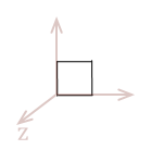
We need a frame of reference that can be used as the eye or camera. We call this frame of reference the view space and the eye is located at the view-point. In fact, up to this point we have also used two other vector-spaces, local space (also called model space and world space. To be able to create our projection transformation, we need to introduce one last coordinate space called screen space. Screen space is a 2D coordinate system defined by the \(uv-plane\), and it maps directly to the display image or screen.
The diagram below depicts all four of these different coordinate spaces:
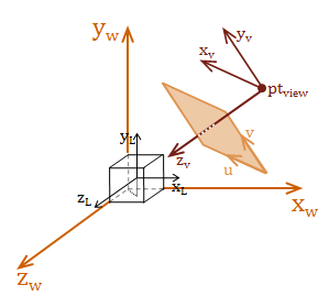
The important concept to understand, is that all of these coordinate systems are relatively positioned, scaled, and oriented to each other. We construct our transforms to move between these coordinate spaces. To render a view of the scene, we need to construct a transform to go from world space to view space.
View Space
The view space is the frame of reference for the eye. Basically, our view of the scene. This coordinate space allows us to transform the world coordinates to a position relative to our view point. This makes it possible for us to create a projection of this visible scene onto our view plane.
We need a point and two vectors to define the location and orientation of the view space. The method I demonstrate here is called the "eye, at, up" method. This is because we specify a point to be the location of the eye, a vector from the eye to the focal-point, at, and a vector that indicates which direction is up. I like this method because I think it is an intuitive model for visualizing where your view-point is located, how it is oriented, and what you are looking at.
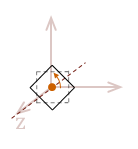
Right or Left Handed?
The view space is a left-handed coordinate system, which differs from the right-handed coordinate systems that we have used up to this point. In math and physics, right-handed systems are the norm. This places the \(y-axis\) up, and the \(x-axis\) pointing to the right (same as the classic 2D Cartesian grid), and the resulting \(z-axis\) will point toward you. For a left-handed space, the positive \(z-axis\) points into the paper. This makes things very convenient in computer graphics, because \(z\) is typically used to measure and indicate depth.
You can tell which type of coordinate system that you have created by taking your open palm and pointing it perpendicularly to the \(x-axis\), and your palm facing the \(y-axis\). The positive \(z-axis\) will point in the direction of your thumb, based upon the direction your coordinate space is oriented.
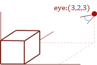
Let's define a simple view space transformation.
\( \eqalign{ eye&= [\matrix{2 & 3 & 3}] \\ at&= [\matrix{0 & 0 & 0}] \\ up&= [\matrix{0 & 1 & 0}] }\)
Simple Indeed.
From this, we can create a view located at \([\matrix{2 & 3 & 3}]\) that is looking at the origin and is oriented vertically (no tilt to either side). We start by using the vector operations, which I demonstrated in my previous post, to define vectors for each of the three coordinate axes.
\( \eqalign{ z_{axis}&= \| at-eye \| \\ &= \| [\matrix{-2 & -3 & -3}] \| \\ &= [\matrix{-0.4264 & -0.6396 & -0.6396}] \\ \\ x_{axis}&= \| up \times z_{axis} \| \\ &=\| [\matrix{-3 & 0 & 2}] \|\\ &=[\matrix{-0.8321 & 0 & 0.5547}]\\ \\ y_{axis}&= \| z_{axis} \times x_{axis} \| \\ &= [\matrix{-0.3547 & -0.7687 & -0.5322}] }\)
We now take these three vectors, and plug them into this composite matrix that is designed to transform world space to a new coordinate space defined by axis-aligned unit vectors.
\( \eqalign { T_{view}&=\left\lbrack \matrix{ x_{x_{axis}} & x_{y_{axis}} & x_{z_{axis}} & 0 \\ y_{x_{axis}} & y_{y_{axis}} & y_{z_{axis}} & 0 \\ z_{x_{axis}} & z_{y_{axis}} & z_{z_{axis}} & 0 \\ -(x_{axis} \cdot eye) & -(y_{axis} \cdot eye) & -(z_{axis} \cdot eye) & 1 \\ } \right\rbrack \\ \\ &=\left\lbrack \matrix{ -0.8321 & -0.3547 & -0.4264 & 0 \\ 0 & -0.7687 & -0.6396 & 0 \\ -0.5547 & -0.5322 & -0.6396 & 0 \\ 3.3283 & 4.6121 & 4.6904 & 1 \\ } \right\rbrack }\)
Gaining Perspective
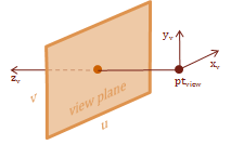
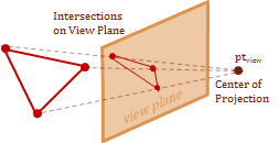
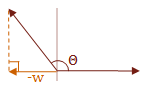
The final step is to project what we can see from the \(eye\) in our view space, onto the view-plane. As I mentioned previous, the view-plane is commonly referred to as the \(uv-plane\). The \(uv\) coordinate-system refers to the 2D mapping on the \(uv-plane\). The projection mapping that I demonstrate here places the \(uv-plane\) some distance \(d\) from the \(eye\), so that the view-space \(z-axis\) is parallel with the plane's normal.
The \(eye\) is commonly referred to by another name for the context of the projection transform, it is called the center of projection. That is because this final step, basically, projects the intersection of a projected vector onto the \(uv-plane\). The projected vector originates at the center of projection and points to each point in the view-space.
The cues that let us perceive perspective with stereo-scopic vision is called, fore-shortening. This effect is caused by objects appearing much smaller as they are further from our vantage-point. Therefore, we can recreate the foreshortening in our image by scaling the \(xy\) values based on their \(z\)-coordinate. Basically, the farther away an object is placed from the center of projection, the smaller it will appear.
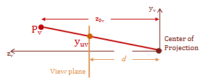
The diagram above shows a side view of the \(y\) and \(z\) axes, and is parallel with the \(x-axis\). Notice the have similar triangles that are created by the view plane. The smaller triangle on the bottom is the distance \(d\), which is the distance from the center of projection to the view plane. The larger triangle on the top extends from the point \(Pv\) to the \(y-axis\), this distance is the \(z\)-component value for the point \(Pv\). Using the property of similar triangles we now have a geometric relationship that allows us to scale the location of the point for the view plane intersection.
|
\(\frac{x_s}d = \frac{x_v}{z_v}\) |
\(\frac{y_s}d = \frac{y_v}{z_v}\) |
|
\(x_s = \frac{x_v}{z_v/d}\) |
\(y_s = \frac{y_v}{z_v/d}\) |
With this, we can define a perspective-based projection transform:
\( T_{project}=\left\lbrack \matrix{ 1 & 0 & 0 & 0 \\ 0 & 1 & 0 & 0 \\ 0 & 0 & 1 & 1/d \\ 0 & 0 & 0 & 0} \right\rbrack \)
This is now where the homogenizing component \(w\) returns. This transform will have the affect of scaling the \(w\) component to create:
\( \eqalign{ X&= x_v \\ Y&= y_v \\ Z&= z_v \\ w&= z_v/d }\)
Which is why we need to access these values as shown below after the following transform is used:
\( \eqalign{ [\matrix{X & Y & Z & w}] &= [\matrix{x_v & y_v & z_v & 1}] T_{project}\\ \\ x_v&= X/w \\ y_v&= Y/w \\ z_v&= Z/w }\)
Scale the Image Plane
Here is one last piece of information that I think you will appreciate. The projection transform above defines a \(uv\) coordinate system that is \(1 \times 1\). Therefore, if you make the following adjustment, you will scale the unit-plane to match the size of your final image in pixels:
\( T_{project}=\left\lbrack \matrix{ width & 0 & 0 & 0 \\ 0 & height & 0 & 0 \\ 0 & 0 & 1 & 1/d \\ 0 & 0 & 0 & 0} \right\rbrack \)
Summary
We made it! With a little bit of knowledge from both Linear Algebra and Trigonometry, we have been able to construct and manipulate geometric models in 3D space, concatenate transform matrices into compact and efficient transformation definitions, and finally create a projection transform to create a two-dimensional image from a three-dimensional definition.
As you can probably guess, this is only the beginning. There is so much more to explore in the creation of computer graphics. Some of the more interesting topics that generally follow after the 3D projection is created are:
- Shading Models: Flat, Gouraud and Phong.
- Shadows
- Reflections
- Transparency and Refraction
- Textures
- Bump-mapping ...
The list goes on and on. I imagine that I will continue to write on this topic and address polygon fill algorithms and the basic shading models. However, I think things will be more interesting if I have code to demonstrate and possibly an interactive viewer for the browser. I have a few demonstration programs written in C++ for Windows, but I would prefer to create something that is a bit more portable.
Once I decide how I want to proceed I will return to this topic. However, if enough people express interest, I wouldn't mind continuing forward demonstrating with C++ Windows programs. Let me know what you think.
References
Watt, Alan, "Three-dimensional geometry in computer graphics," in 3D Computer Graphics, Harlow, England: Addison-Wesley, 1993
Foley, James, D., et al., "Geometrical Transformations," in Computer Graphics: Principles and Practice, 2nd ed. in C, Reading: Addison-Wesley, 1996
I previously introduced how to perform the basic matrix operations commonly used in 3D computer graphics. However, we haven’t yet reached anything that resembles graphics. I now introduce the concepts of geometry as it’s related to computer graphics. I intend to provide you with the remaining foundation necessary to be able to mathematically visualize the concepts at work. Unfortunately, we will still not be able to reach the "computer graphics" stage with this post; that must wait until the next entry.
This post covers a basic form of a polygonal mesh to represent models, points and Euclidean vectors. With the previous entry and this one, we will have all of the background necessary for me to cover matrix transforms in the next post. Specifically the 3D projection transform, which provides the illusion of perspective. This will be everything that we need to create a wireframe viewer. For now, let's focus on the topics of this post.
Modeling the Geometry
We will use models composed of a mesh of polygons. All of the polygons will be defined as triangles. It is important to consistently define the points of each triangle either clockwise or counter-clockwise. This is because the definition order affects the direction a surface faces. If a single model mixes the order of point definitions, your rendering will have missing polygons.
The order of point definition for the triangle can be ignored if a surface normal is provided for each polygon. However, to keep things simple, I will only be demonstrating with basic models that are built from an index array structure. This data structure contains two arrays. The first array is a list of all of the vertices (points) in the model. The second array contains a three-element structure with the index of the point that can be found in the first array. I define all of my triangles counter-clockwise while looking at the front of the surface.
Generally, your models should be defined at or near the origin. The rotation transformation that we will explore in the next post requires a pivot point, which is defined at the origin. Model geometries defined near the origin are also easier to work with when building models from smaller components and using instancing to create multiple copies of a single model.
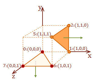
Here is a definition for a single triangle starting at the origin and adjacent to the Y plane. The final corner decreases for Y as it moves diagonally along the XZ plane:
|
|
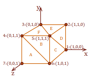
This definition represents a unit cube starting at the origin. A cube has 8 corners to hold six square-faces. It requires two triangles to represent each square. Therefore, there are 8 points used to define 12 triangles:
|
|
Vectors
Recall from my previous post that a vector is a special type of matrix, in which there is only a single row or column. You may be aware of a different definition for the term "vector"; something like
NOUN
A quantity having direction as well as magnitude, especially determining the position of one point in space relative to another.
Oxford Dictionary
From this point forward, when I use the term "vector", I mean a Euclidean vector. We will even use single-row and single-column matrices to represent these vectors; we’re just going to refer to those structures as matrices to minimize the confusion.
Notational Convention
It is most common to see vectors represented as single-row matrices, as opposed to the standard mathematical notation which uses column matrices to represent vectors. It is important to remember this difference in notation based on what type of reference you are following.
The reason for this difference, is the row-form makes composing the transformation matrix more natural as the operations are performed left-to-right. I discuss the transformation matrix in the next entry. As you will see, properly constructing transformation matrices is crucial to achieve the expected results, and anything that we can do to simplify this sometimes complex topic, will improve our chances of success.
Representation
As the definition indicates, a vector has a direction and magnitude. There is a lot of freedom in that definition for representation, because it is like saying "I don’t know where I am, but I know which direction I am heading and how far I can go." Therefore, if we think of our vector as starting at the origin of a Cartesian grid, we could then represent a vector as a single point.
This is because starting from the origin, the direction of the vector is towards the point. The magnitude can be calculated by using Pythagoras' Theorem to calculate the distance between two points. All of this information can be encoded in a compact, single-row matrix. As the definition indicates, we derive a vector from two points, by subtracting one point from the other using inverse of matrix addition.
This will give us the direction to the destination point, relative to the starting point. The subtraction effectively acts as a translation of the vectors starting point to the origin.
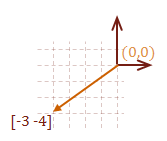
For these first few vector examples, I am going to use 2D vectors. Because they are simpler to demonstrate and diagram, and the only difference to moving to 3D vectors is an extra field has been added.
Here is a simple example with two points (2, 1) and (5, 5). The first step is to encode them in a matrix:
\( {\bf S} = \left\lbrack \matrix{2 & 1} \right\rbrack, {\bf D} = \left\lbrack \matrix{5 & 5} \right\rbrack \)
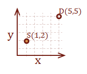
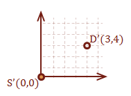
Let’s create two vectors, one that determines how to get to point D starting from S, and one to get to point S starting from D. The first step is to subtract the starting point from the destination point. Notice that if we were to subtract the starting point from itself, the result is the origin, (0, 0).
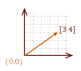
\( \eqalign{ \overrightarrow{SD} &= [ \matrix{5 & 5} ] - [ \matrix{2 & 1} ] \cr &= [ \matrix{3 & 4} ] } \)
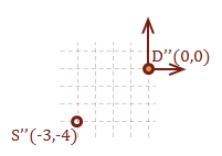
\( \eqalign{ \overrightarrow{DS} &= [ \matrix{2 & 1} ] - [ \matrix{5 & 5} ] \cr &= [ \matrix{-3 & -4} ] } \)
Notice that the only difference between the two vectors is the direction. The magnitude of each vector is the same, as expected. Here is how to calculate the magnitude of a vector:
Given:
\( \eqalign{ v &= \matrix{ [a_1 & a_2 & \ldots & a_n]} \cr |v| &= \sqrt{\rm (a_1^2 + a_2^2 + \ldots + a_n^2)} } \)
Operations
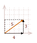
I covered scalar multiplication and matrix addition in my previous post. However, I wanted to briefly revisit the topic to demonstrate one way to think about vectors, which may help you develop a better intuition for the math. For the coordinate systems that we are working with, vectors are straight lines.
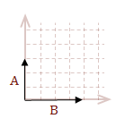
When you add two or more vectors together, you can think of them as moving the tail of each successive vector to the head of the previous vector. Then add the corresponding components.
\( \eqalign{ v &= A+B \cr |v| &= \sqrt{\rm 3^2 + 4^2} \cr &= 5 }\)
Regardless of the orientation of the vector, it can be decomposed into its individual contributions per axis. In our model for the vector, the contribution for each axis is the raw value defined in our matrix.
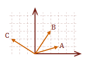
\( v = A+B+C \)
\( \eqalign{ |v| &= \sqrt{\rm (3+2-3)^2 + (1+3+2)^2} \cr &= \sqrt{\rm 2^2 + 6^2} \cr &= 2 \sqrt{\rm 10} }\)
Unit Vector
We can normalize a vector to create unit vector, which is a vector that has a length of 1. The concept of the unit vector is introduced to reduce a vector to simply indicate its direction. This type of vector can now be used as a unit of measure to which other vectors can be compared. This also simplifies the task of deriving other important information when necessary.
To normalize a vector, divide the vector by its magnitude. In terms of the matrix operations that we have discussed, this is simply scalar multiplication of the vector with the inverse of its magnitude.
\( u = \cfrac{v}{ |v| } \)
\(u\) now contains the information for the direction of \(v\). With algebraic manipulation we can also have:
\( v = u |v| \)
This basically says the vector \(v\) is equal to the unit vector that has the direction of \(u\) multiplied by the magnitude of \(v\).
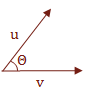
Dot Product
The dot product is used for detecting visibility and shading of a surface. The dot product operation is shown below:
\( \eqalign{ w &= u \cdot v \cr &= u_1 v_1 + u_2 v_2 + \cdots + u_n v_n }\)
This formula may look familiar. That is because this is a special case in matrix multiplication called the inner product, which looks like this (remember, we are representing vectors as a row matrix):
\( \eqalign{ u \cdot v &= u v^T \cr &= \matrix {[u_1 & u_2 & \cdots & u_n]} \left\lbrack \matrix{v_1 \\ v_2 \\ \vdots \\ v_n } \right\rbrack }\)
We will use the dot product on two unit vectors to help us determine the angle between these vectors; that’s right, angle. We can do this because of the cosine rule from Trigonometry. The equation that we can use is as follows:
\( \cos \Theta = \cfrac{u \cdot v} {|u||v|} \)
To convert this to the raw angle, \(\Theta\), you can use the inverse function of cosine, arccos(\( \Theta \)). In C and C++ the name of the function is acos().
\( \cos {\arccos \Theta} = \Theta \)
So what is actually occurring when we calculate the dot product that allows us to get an angle?
We are essentially calculating the projection of u onto v. This gives us enough information to manipulate the Trigonometric properties to derive \( \Theta \).

I would like to make one final note regarding the dot product. Many times it is only necessary to know the sign of the angle between two vectors. The following table shows the relationship between the dot product of two vectors and the value of the angle, \( \Theta \), which is in the range \( 0° \text{ to } 180° \). If you like radians, that is \( 0 \text{ to } \pi \).
\( w = u \cdot v = f(u,w) \)
\( f(u,w) = \cases{ w \gt 0 & \text { if } \Theta \lt 90° \cr w = 0 & \text { if } \Theta = 90° \cr w \lt 0 & \text { if } \Theta \gt 90° }\)
Cross Product
The cross product is used to calculate a vector that is perpendicular to a surface. The name for this vector is the surface normal. The surface normal indicates which direction the surface is facing. Therefore, it is used quite extensively for shading and visibility as well.
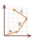
We have reached the point where we need to start using examples and diagrams with three dimensions. We will use the three points that define our triangular surface to create two vectors. Remember, it is important to use consistent definitions when creating models.
The first step is to calculate our planar vectors. What does that mean? We want to create two vectors that are coplanar (on the same plane), so that we may use them to calculate the surface normal. All that we need to be able to do this are three points that are non-collinear, and we have this with each triangle definition in our polygonal mesh model.
If we have defined a triangle \(\triangle ABC\), we will define two vectors, \(u = \overrightarrow{AB}\) and \(v = \overrightarrow{AC}\).
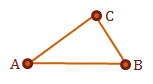
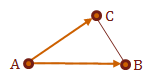
If we consistently defined the triangle surfaces in our model, we should now be able to take the cross product of \(u \times v\) to receive the surface normal, \(N_p\), of \(\triangle ABC\). Again, the normal vector is perpendicular to its surface.
In practice, this tells us which direction the surface is facing. We would combine this with the dot product to help us determine if are interested in this surface for the current view.
So how do you calculate the cross product?
Here is what you need to know in order to calculate the surface normal vector:
\(\eqalign { N_p &= u \times v \cr &= [\matrix{(u_2v_3 – u_3v_2) & (u_3v_1 – u_1v_3) & (u_1v_2 – u_2v_1)}] }\)
To help you remember how to perform the calculation, I have re-written it in parts, and used \(x\), \(y\), and \(z\) rather than the index values.
\(\eqalign { x &= u_yv_z – u_zv_y \cr y &= u_zv_x – u_xv_z \cr z &= u_xv_y – u_yv_x }\)
Let's work through an example to demonstrate the cross product. We will use surface A from our axis-aligned cube model that we constructed at the beginning of this post. Surface A is defined completely within the XY plane. How do we know this? Because all of the points have the same \(z\)-coordinate value of 1. Therefore, we should expect that our calculation for \(N_p\) of surface A will be an \(z\) axis-aligned vector pointing in the positive direction.
Step 1: Calculate our surface description vectors \(u\) and \(v\):
\( Surface_A = pt_7: (0,0,1), pt_6: (1,0,1), \text{ and } pt_4: (0,1,1) \)
|
\( \eqalign { u &= pt_6 - pt_7 \cr &= [\matrix{1 & 0 & 1}] - [\matrix{0 & 0 & 1}] \cr &=[\matrix{\color{red}{1} & \color{green}{0} & \color{blue}{0}}] }\) |
\( \eqalign { v &= pt_4 - pt_7 \cr &= [\matrix{0 & 1 & 1}] - [\matrix{0 & 0 & 1}] \cr &=[\matrix{\color{red}{0} & \color{green}{1} & \color{blue}{0}}] }\) |
Step 2: Calculate \(u \times v\):
\(N_p = [ \matrix{x & y & z} ]\text{, where:}\)
|
\( \eqalign { x &= \color{green}{u_y}\color{blue}{v_z} – \color{blue}{u_z}\color{green}{v_y} \cr &= \color{green}{0} \cdot \color{blue}{0} - \color{blue}{0} \cdot \color{green}{1} \cr &= 0 }\) |
\( \eqalign { y &= \color{blue}{u_z}\color{red}{v_x} – \color{red}{u_x}\color{blue}{v_z} \cr &= \color{blue}{0} \cdot \color{red}{0} - \color{red}{1} \cdot \color{blue}{0} \cr &= 0 }\) |
\( \eqalign { z &= \color{red}{u_x}\color{green}{v_y} – \color{green}{u_y}\color{red}{v_x} \cr &= \color{red}{1} \cdot \color{green}{1} - \color{green}{0} \cdot \color{red}{0} \cr &= 1 }\) |
\(N_p = [ \matrix{0 & 0 & 1} ]\)
This is a \(z\) axis-aligned vector pointing in the positive direction, which is what we expected to receive.
Notation Formality
If you look at other resources to learn more about the cross product, it is actually defined as a sum in terms of three axis-aligned vectors \(i\), \(j\), and \(k\), which then must be multiplied by the vectors \(i=[\matrix{1&0&0}]\), \(j=[\matrix{0&1&0}]\), and \(k=[\matrix{0&0&1}]\) to get the final vector. The difference between what I presented and the form with the standard vectors, \(i\), \(j\), and \(k\), is I omitted a step by placing the result calculations directly in a new vector. I wanted you to be aware of this discrepancy between what I have demonstrated and what is typically taught in the classroom.
Apply What We Have Learned
We have discovered quite a few concepts between the two posts that I have written regarding the basic math and geometry involved with computer graphics. Let's apply this knowledge and solve a useful problem. Detecting if a surface is visible from a specific point-of-view is a fundamental problem that is used extensively in this domain. Since we have all of the tools necessary to solve this, let's run through two examples.
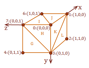
For the following examples we will specify the view-point as \(pt_{eye} = [\matrix{3 & 2 & 3}]:\)
Also, refer to this diagram for the surfaces that we will test for visibility from the view-point. The side surface is surface \(D\) from the cube model, and the hidden surface is the bottom-facing surface \(J\).
Detect a visible surface
Step 1: Calculate our surface description vectors \(u\) and \(v\):
\( \eqalign{ Surface_D: &pt_5: (1,1,1), \cr &pt_1: (1,0,0), \cr &pt_2: (1,1,0) } \)
|
\( \eqalign { u &= pt_1 - pt_5 \cr &= [\matrix{1 & 0 & 0}] - [\matrix{1 & 1 & 1}] \cr &=[\matrix{0 & -1 & -1}] }\) |
\( \eqalign { v &= pt_2 - pt_5 \cr &= [\matrix{1 & 1 & 0}] - [\matrix{1 & 1 & 1}] \cr &=[\matrix{0 & 0 & -1}] }\) |
Step 2: Calculate \(u \times v\):
\(N_{pD} = [ \matrix{x & y & z} ]\text{, where:}\)
|
\( \eqalign { x &= -1 \cdot (-1) - (-1) \cdot 0 \cr &= 1 }\) |
\( \eqalign { y &= -1 \cdot 0 - (-1) \cdot 0 \cr &= 0 }\) |
\( \eqalign { z &= 0 \cdot 0 - (-1) \cdot 0 \cr &= 0 }\) |
\(N_pD = [ \matrix{1 & 0 & 0} ]\)
Step 3: Calculate vector to the eye:
To calculate a vector to the eye, we need to select a point on the target surface and create a vector to the eye. For this example, we will select \(pt_5\)
\( \eqalign{ \overrightarrow{view_D} &= pt_{eye} - pt_5\cr &= [ \matrix{3 & 2 & 3} ] - [ \matrix{1 & 1 & 1} ]\cr &= [ \matrix{2 & 1 & 2} ] }\)
Step 4: Normalize the view-vector:
Before we can use this vector in a dot product, we must normalize the vector:
\( \eqalign{ |eye_D| &= \sqrt{\rm 2^2 + 1^2 + 2^2} \cr &= \sqrt{\rm 4 + 1 + 4} \cr &= \sqrt{\rm 9} \cr &= 3 \cr \cr eye_u &= \cfrac{eye_D}{|eye_D|} \cr &= \cfrac{1}3 [\matrix{2 & 1 & 2}] \cr &= \left\lbrack\matrix{\cfrac{2}3 & \cfrac{1}3 & \cfrac{2}3} \right\rbrack }\)
Step 5: Calculate the dot product of the view-vector and surface normal:
\( \eqalign{ w &= eye_{u} \cdot N_{pD} \cr &= \cfrac{2}3 \cdot 1 + \cfrac{1}3 \cdot 0 + \cfrac{2}3 \cdot 0 \cr &= \cfrac{2}3 }\)
Step 6: Test for visibility:
|
\(w \gt 0\), therefore \(Surface_D\) is visible. |
|
Detect a surface that is not visible
Step 1: Calculate our surface description vectors \(u\) and \(v\):
\( \eqalign{ Surface_J: &pt_6: (1,1,1), \cr &pt_0: (0,0,0), \cr &pt_1: (1,0,0) } \)
|
\( \eqalign { u &= pt_0 - pt_6 \cr &= [\matrix{0 & 0 & 0}] - [\matrix{1 & 0 & 1}] \cr &=[\matrix{-1 & 0 & -1}] }\) |
\( \eqalign { v &= pt_1 - pt_6 \cr &= [\matrix{1 & 0 & 0}] - [\matrix{1 & 0 & 1}] \cr &=[\matrix{0 & 0 & -1}] }\) |
Step 2: Calculate \(u \times v\):
\(N_{pJ} = [ \matrix{x & y & z} ]\text{, where:}\)
|
\( \eqalign { x &= 0 \cdot (-1) - (-1) \cdot 0 \cr &= 0 }\) |
\( \eqalign { y &= -1 \cdot 0 - (-1) \cdot (-1) \cr &= -1 }\) |
\( \eqalign { z &= (-1) \cdot 0 - 0 \cdot 0 \cr &= 0 }\) |
\(N_pJ = [ \matrix{0 & -1 & 0} ]\)
Step 3: Calculate vector to the eye:
For this example, we will select \(pt_6\)
\( \eqalign{ \overrightarrow{view_J} &= pt_{eye} - pt_6\cr &= [ \matrix{3 & 2 & 3} ] - [ \matrix{1 & 0 & 1} ]\cr &= [ \matrix{2 & 2 & 2} ] }\)
Step 4: Normalize the view-vector:
Before we can use this vector in a dot product, we must normalize the vector:
\( \eqalign{ |eye_J| &= \sqrt{\rm 2^2 + 2^2 + 2^2} \cr &= \sqrt{\rm 4 + 4 + 4} \cr &= \sqrt{\rm 12} \cr &= 2 \sqrt{\rm 3} \cr \cr eye_u &= \cfrac{eye_J}{|eye_J|} \cr &= \cfrac{1}{2 \sqrt 3} [\matrix{2 & 2 & 2}] \cr &= \left\lbrack\matrix{\cfrac{1}{\sqrt 3} & \cfrac{1}{\sqrt 3} & \cfrac{1}{\sqrt 3}} \right\rbrack }\)
Step 5: Calculate the dot product of the view-vector and surface normal:
\( \eqalign{ w &= eye_{u} \cdot N_{pJ} \cr &= \cfrac{1}{\sqrt 3} \cdot 0 + \cfrac{1}{\sqrt 3} \cdot (-1) + \cfrac{1}{\sqrt 3} \cdot 0 \cr &= -\cfrac{1}{\sqrt 3} }\)
Step 6: Test for visibility:
|
\(w \lt 0\), therefore \(Surface_J\) is not visible. |
|
What has this example demonstrated?
Surprisingly, this basic task demonstrates every concept that we have learned from the two posts up to this point:
- Matrix Addition: Euclidean vector creation
- Scalar Multiplication: Unit vector calculation, multiplying by \(1 / |v| \).
- Matrix Multiplication: Dot Product calculation, square-matrix multiplication will be used in the next post.
- Geometric Model Representation: The triangle surface representation provided the points for our calculations.
- Euclidean Vector: Calculation of each surfaces planar vectors, as well as the view vector.
- Cross Product: Calculation of the surface normal, \(N_p\).
- Unit Vector: Preparation of vectors for dot product calculation.
- Dot Product: Used the sign from this calculation to test for visibility of a surface.
Summary
Math can be difficult sometimes, especially with all of the foreign notation. However, with a bit of practice the notation will soon become second nature and many calculations can be performed in your head, similar to basic arithmetic with integers. While many graphics APIs hide these calculations from you, don't be fooled because they still exist and must be performed to display the three-dimensional images on your screen. By understanding the basic concepts that I have already demonstrated, you will be able to better troubleshoot your graphics programs when something wrong occurs. Even if you rely solely on a graphics library to abstract the complex mathematics.
There is only one more entry to go, and we will have enough basic knowledge of linear algebra, Euclidean geometry, and computer displays to be able to create, manipulate and display 3D models programmatically. The next entry discusses how to translate, scale and rotate geometric models. It also describes what must occur to create the illusion of a three-dimensional image on a two-dimensional display with the projection transform.
References
Watt, Alan, "Three-dimensional geometry in computer graphics," in 3D Computer Graphics, Harlow, England: Addison-Wesley, 1993
Three-dimensional computer graphics is an exciting aspect of computing because of the amazing visual effects that can be created for display. All of this is created from an enormous number of calculations that manipulate virtual models, which are constructed from some form of geometric definition. While the math involved for some aspects of computer graphics and animation can become quite complex, the fundamental mathematics that is required is very accessible. Beyond learning some new mathematic notation, a basic three-dimensional view can be constructed with algorithms that only require basic arithmetic and a little bit of trigonometry.
I demonstrate how to perform some basic operations with two key constructs for 3D graphics, without the rigorous mathematic introduction. Hopefully the level of detail that I use is enough for anyone that doesn't have a strong background in math, but would very much like to play with 3D APIs. I introduce the math that you must be familiar with in this entry, and in two future posts I demonstrate how to manipulate geometric models and apply the math towards the display of a 3D image.
Linear Algebra
The type of math that forms the basis of 3D graphics is called linear algebra. In general, linear algebra is quite useful for solving systems of linear equations. Rather than go into the details of linear algebra, and all of its capabilities, we are going to simply focus on two related constructs that are used heavily within the topic, the matrix and the vertex.
Matrix
The Matrix provides an efficient mechanism to translate, scale, rotate, and convert between different coordinate systems. This is used extensively to manipulate the geometric models for environment calculations and display.
These are all examples of valid matrices:
\( \left\lbrack \matrix{a & b & c \cr d & e & f} \right\rbrack, \left\lbrack \matrix{10 & -27 \cr 0 & 13 \cr 7 & 17} \right\rbrack, \left\lbrack \matrix{x^2 & 2x \cr 0 & e^x} \right\rbrack\)
Square matrices are particularly important, that is a matrix with the same number of columns and rows. There are some operations that can only be performed on a square matrix, which I will introduce shortly. The notation for matrices, in general, uses capital letters as the variable names. Matrix dimensions can be specified as a shorthand notation, and to also identify an indexed position within the matrix. As far as I am aware, row-major indexing is always used for consistency, that is, the first index represents the row, and the second represents the column.
\( A= [a_{ij}]= \left\lbrack \matrix{a_{11} & a_{12} & \ldots & a_{1n} \cr a_{21} & a_{22} & \ldots & a_{2n} \cr \vdots & \vdots & \ddots & \vdots \cr a_{m1} & a_{m2} & \ldots & a_{mn} } \right\rbrack \)
Vector
The vector is a special case of a matrix, where there is only a single row or a single column; also a common practice is to use lowercase letters to represent vectors:
\( u= \left\lbrack \matrix{u_1 & u_2 & u_3} \right\rbrack \), \( v= \left\lbrack \matrix{v_1\cr v_2\cr v_3} \right\rbrack\)
Operations
The mathematical shorthand notation for matrices is very elegant. It simplifies these equations that would be quite cumbersome, otherwise. There are only a few operations that we are concerned with to allow us to get started. Each operation has a basic algorithm to follow to perform a calculation, and the algorithm easily scales with the dimensions of a matrix.
Furthermore, the relationship between math and programming is not always clear. I have a number of colleagues that are excellent programmers and yet they do not consider their math skills very strong. I think that it could be helpful to many to see the conversion of the matrix operations that I just described from mathematical notation into code form. Once I demonstrate how to perform an operation with the mathematical notation and algorithmic steps, I will also show a basic C++ implementation of the concept to help you understand how these concepts map to actual code.
The operations that I implement below assume a Matrix class with the following interface:
C++
class Matrix | |
{ | |
public: | |
// Ctor and Dtor omitted | |
| |
// Calculate and return a reference to the specified element. | |
double& element(size_t row, size_t column); | |
| |
// Resizes this Matrix to have the specified size. | |
void resize(size_t row, size_t column); | |
| |
// Returns the number rows. | |
size_t rows(); | |
| |
// Returns the number of columns. | |
size_t columns(); | |
private: | |
std::vector<double> data; | |
}; |
Transpose
Transpose is a unary operation that is performed on a single matrix, and it is represented by adding a superscript T to target matrix.
For example, the transpose of a matrix A is represented with AT.
The transpose "flips" the orientation of the matrix so that each row becomes a column, and each original column is transformed into a row. I think that a few examples will make this concept more clear.
\( A= \left\lbrack \matrix{a & b & c \cr d & e & f \cr g & h & i} \right\rbrack \)
\(A^T= \left\lbrack \matrix{a & d & g \cr b & e & h \cr c & f & i} \right\rbrack \)
The resulting matrix will contain the same set of values as the original matrix, only their position in the matrix changes.
\( B= \left\lbrack \matrix{1 & 25 & 75 & 100\cr 0 & 5 & -50 & -25\cr 0 & 0 & 10 & 22} \right\rbrack \)
\(B^T= \left\lbrack \matrix{1 & 0 & 0 \cr 25 & 5 & 0 \cr 75 & -50 & 10 \cr 100 & -25 & 22} \right\rbrack \)
It is very common to transpose a matrix, including vertices, before performing other operations. The reason will become clear for matrix multiplication.
\( u= \left\lbrack \matrix{u_1 & u_2 & u_3} \right\rbrack \)
\(u^T= \left\lbrack \matrix{u_1 \cr u_2 \cr u_3} \right\rbrack \)
Matrix Addition
Addition can only be performed between two matrices that are the same size. By size, we mean that the number of rows and columns are the same for each matrix. Addition is performed by adding the values of the corresponding positions of both matrices. The sum of the values creates a new matrix that is the same size as the original two matrices provided to the add operation.
If
\( A= \left\lbrack \matrix{0 & -2 & 4 \cr -6 & 8 & 0 \cr 2 & -4 & 6} \right\rbrack, B= \left\lbrack \matrix{1 & 3 & 5 \cr 7 & 9 & 11 \cr 13 & 15 & 17} \right\rbrack \)
Then
\(A+B=\left\lbrack \matrix{1 & 1 & 9 \cr 1 & 17 & 11 \cr 15 & 11 & 23} \right\rbrack \)
The size of these matrices do not match in their current form.
\(U= \left\lbrack \matrix{4 & -8 & 5}\right\rbrack, V= \left\lbrack \matrix{-1 \\ 5 \\ 4}\right\rbrack \)
However, if we take the transpose of one of them, their sizes will match and they can then be added together. The size of the result matrix depends upon which matrix we perform the transpose operation on from the original expression.:
\(U^T+V= \left\lbrack \matrix{3 \\ -3 \\ 9} \right\rbrack \)
Or
\(U+V^T= \left\lbrack \matrix{3 & -3 & 9} \right\rbrack \)
Matrix addition has the same algebraic properties as with the addition of two scalar values:
Commutative Property:
Associative Property:
Identity Property:
Inverse Property:
The code required to implement matrix addition is relatively simple. Here is an example for the Matrix class definition that I presented earlier:
C++
void Matrix::operator+=(const Matrix& rhs) | |
{ | |
if (rhs.data.size() == data.size()) | |
{ | |
// We can simply add each corresponding element | |
// in the matrix element data array. | |
for (size_t index = 0; index < data.size(); ++index) | |
{ | |
data[index] += rhs.data[index]; | |
} | |
} | |
} | |
| |
Matrix operator+( const Matrix& lhs, | |
const Matrix& rhs) | |
{ | |
Matrix result(lhs); | |
result += rhs; | |
| |
return result; | |
} |
Scalar Multiplication
Scalar multiplication allows a single scalar value to be multiplied with every entry within a matrix. The result matrix is the same size as the matrix provided to the scalar multiplication expression:
If
\( A= \left\lbrack \matrix{3 & 6 & -9 \cr 12 & -15 & -18} \right\rbrack \)
Then
\( \frac{1}3 A= \left\lbrack \matrix{1 & 2 & -3 \cr 4 & -5 & -6} \right\rbrack, 0A= \left\lbrack \matrix{0 & 0 & 0 \cr 0 & 0 & 0} \right\rbrack, -A= \left\lbrack \matrix{-3 & -6 & 9 \cr -12 & 15 & 18} \right\rbrack, \)
Scalar multiplication with a matrix exhibits these properties, where c and d are scalar values:
Distributive Property:
Identity Property:
The implementation for scalar multiplication is even simpler than addition.
Note: this implementation only allows the scalar value to appear before the Matrix object in multiplication expressions, which is how the operation is represented in math notation.:
C++
void Matrix::operator*=(const double lhs) | |
{ | |
for (size_t index = 0; index < data.size(); ++index) | |
{ | |
data[index] *= rhs; | |
} | |
} | |
| |
Matrix operator*( const double scalar, | |
const Matrix& rhs) | |
{ | |
Matrix result(rhs); | |
result *= scalar; | |
| |
return result; | |
} |
Matrix Multiplication
Everything seems very simple with matrices, at least once you get used to the new structure. Then you are introduced to matrix multiplication. The algorithm for multiplication is not difficult, however, it is much more labor intensive compared to the other operations that I have introduced to you. There are also a few more restrictions on the parameters for multiplication to be valid. Finally, unlike the addition operator, the matrix multiplication operator does not have all of the same properties as the multiplication operator for scalar values; specifically, the order of parameters matters.
Input / Output
Let's first address what you need to be able to multiply matrices, and what type of matrix you can expect as output. Once we have addressed the structure, we will move on to the process.
Given an the following two matrices:
\( A= \left\lbrack \matrix{a_{11} & \ldots & a_{1n} \cr \vdots & \ddots & \vdots \cr a_{m1} & \ldots & a_{mn} } \right\rbrack, B= \left\lbrack \matrix{b_{11} & \ldots & b_{1v} \cr \vdots & \ddots & \vdots \cr b_{u1} & \ldots & b_{uv} } \right\rbrack \)
A valid product for \( AB=C \) is only possible if number of columns \( n \) in \( A \) is equal to the number of rows \( u \) in \( B \). The resulting matrix \( C \) will have the dimensions \( m \times v \).
\( AB=C= \left\lbrack \matrix{c_{11} & \ldots & c_{1v} \cr \vdots & \ddots & \vdots \cr c_{m1} & \ldots & c_{mv} } \right\rbrack, \)
Let's summarize this in a different way, hopefully this arrangement will make the concept more intuitive:

One last form of the rules for matrix multiplication:
- The number of columns, \(n\), in matrix \( A \) must be equal to the number of rows, \(u\), in matrix \( B \):
\( n = u \)
- The output matrix \( C \) will have the number of rows, \(m\), in \(A\), and the number of columns, \(v\), in \(B\):
\( m \times v \)
- \(m\) and \(v\) do not have to be equal. The only requirement is that they are both greater-than zero:
\( m \gt 0,\)
\(v \gt 0 \)
How to Multiply
To calculate a single entry in the output matrix, we must multiply the element from each column in the first matrix, with the element in the corresponding row in the second matrix, and add all of these products together. We use the same row in the first matrix, \(A\), for which we are calculating the row element in \(C\). Similarly, we use the column in the second matrix, \(B\) that corresponds with the calculating column element in \(C\).
More succinctly, we can say we are multiplying rows into columns.
For example:
\( A= \left\lbrack \matrix{a_{11} & a_{12} & a_{13} \cr a_{21} & a_{22} & a_{23}} \right\rbrack, B= \left\lbrack \matrix{b_{11} & b_{12} & b_{13} & b_{14} \cr b_{21} & b_{22} & b_{23} & b_{24} \cr b_{31} & b_{32} & b_{33} & b_{34} } \right\rbrack \)
The number of columns in \(A\) is \(3\) and the number of rows in \(B\) is \(3\), therefore, we can perform this operation. The size of the output matrix will be \(2 \times 4\).
This is the formula to calculate the element \(c_{11}\) in \(C\) and the marked rows used from \(A\) and the columns from \(B\):
\( \left\lbrack \matrix{\color{#B11D0A}{a_{11}} & \color{#B11D0A}{a_{12}} & \color{#B11D0A}{a_{13}} \cr a_{21} & a_{22} & a_{23}} \right\rbrack \times \left\lbrack \matrix{\color{#B11D0A}{b_{11}} & b_{12} & b_{13} & b_{14} \cr \color{#B11D0A}{b_{21}} & b_{22} & b_{23} & b_{24} \cr \color{#B11D0A}{b_{31}} & b_{32} & b_{33} & b_{34} } \right\rbrack = \left\lbrack \matrix{\color{#B11D0A}{c_{11}} & c_{12} & c_{13} & c_{14}\cr c_{21} & c_{22} & c_{23} & c_{24} } \right\rbrack \)
\( c_{11}= (a_{11}\times b_{11}) + (a_{12}\times b_{21}) + (a_{13}\times b_{31}) \)
To complete the multiplication, we need to calculate these other seven values \( c_{12}, c_{13}, c_{14}, c_{21}, c_{22}, c_{23}, c_{24}\). Here is another example for the element \(c_{23}\):
\( \left\lbrack \matrix{ a_{11} & a_{12} & a_{13} \cr \color{#B11D0A}{a_{21}} & \color{#B11D0A}{a_{22}} & \color{#B11D0A}{a_{23}} } \right\rbrack \times \left\lbrack \matrix{b_{11} & b_{12} & \color{#B11D0A}{b_{13}} & b_{14} \cr b_{21} & b_{22} & \color{#B11D0A}{b_{23}} & b_{24} \cr b_{31} & b_{32} & \color{#B11D0A}{b_{33}} & b_{34} } \right\rbrack = \left\lbrack \matrix{c_{11} & c_{12} & c_{13} & c_{14}\cr c_{21} & c_{22} & \color{#B11D0A}{c_{23}} & c_{24} } \right\rbrack \)
\( c_{23}= (a_{21}\times b_{13}) + (a_{22}\times b_{23}) + (a_{23}\times b_{33}) \)
Notice how the size of the output matrix changes. Based on this and the size of the input matrices you can end up with some interesting results:
\( \left\lbrack \matrix{a_{11} \cr a_{21} \cr a_{31} } \right\rbrack \times \left\lbrack \matrix{ b_{11} & b_{12} & b_{13} } \right\rbrack = \left\lbrack \matrix{c_{11} & c_{12} & c_{13} \cr c_{21} & c_{22} & c_{23} \cr c_{31} & c_{32} & c_{33} } \right\rbrack \)
\( \left\lbrack \matrix{ a_{11} & a_{12} & a_{13} } \right\rbrack \times \left\lbrack \matrix{b_{11} \cr b_{21} \cr b_{31} } \right\rbrack = \left\lbrack \matrix{c_{11} } \right\rbrack \)
Tip:
To help you keep track of which row to use from the first matrix and which column from the second matrix, create your result matrix of the proper size, then methodically calculate the value for each individual element.
The algebraic properties for the matrix multiplication operator do not match those of the scalar multiplication operator. These are the most notable:
Not Commutative:
The order of the factor matrices definitely matters.
I think it is very important to illustrate this fact. Here is a simple \(2 \times 2 \) multiplication performed two times with the order of the input matrices switched. I have highlighted the only two terms that the two resulting answers have in common:
\( \left\lbrack \matrix{a & b \cr c & d } \right\rbrack \times \left\lbrack \matrix{w & x\cr y & z } \right\rbrack = \left\lbrack \matrix{(\color{red}{aw}+by) & (ax+bz)\cr (cw+dy) & (cx+\color{red}{dz}) } \right\rbrack \)
\( \left\lbrack \matrix{w & x\cr y & z } \right\rbrack \times \left\lbrack \matrix{a & b \cr c & d } \right\rbrack = \left\lbrack \matrix{(\color{red}{aw}+cx) & (bw+dx)\cr (ay+cz) & (by+\color{red}{dz}) } \right\rbrack \)
Product of Zero:
Scalar Multiplication is Commutative:
Associative Property:
Multiplication is associative, however, take note that the relative order for all of the matrices remains the same.
Transpose of a Product:
The transpose of a product is equivalent to the product of transposed factors multiplied in reverse order
Code
We are going to use a two-step solution to create a general purpose matrix multiplication solution. The first step is to create a function that properly calculates a single element in the output matrix:
C++
double Matrix::multiply_element( | |
const Matrix& rhs, | |
const Matrix& rhs, | |
const size_t i, | |
const size_t j | |
) | |
{ | |
double product = 0; | |
| |
// Multiply across the specified row, i, for the left matrix | |
// and the specified column, j, for the right matrix. | |
// Accumulate the total of the products | |
// to return as the calculated result. | |
for (size_t col_index = 1; col_index <= lhs.columns(); ++col_index) | |
{ | |
for (size_t row_index = 1; row_index <= rhs.rows(); ++row_index) | |
{ | |
product += lhs.element(i, col_index) | |
* rhs.element(row_index, j); | |
} | |
} | |
| |
return product; | |
} |
Now create the outer function that performs the multiplication to populate each field of the output matrix:
C++
// Because we may end up creating a matrix with | |
// an entirely new size, it does not make sense | |
// to have a *= operator for this general-purpose solution. | |
Matrix& Matrix::operator*( const Matrix& lhs, | |
const Matrix& rhs) | |
{ | |
if (lhs.columns() == rhs.rows()) | |
{ | |
// Resize the result matrix to the proper size. | |
this->resize(lhs.row(), rhs.columns()); | |
| |
// Calculate the value for each element | |
// in the result matrix. | |
for (size_t i = 1; i <= this->rows(); ++i) | |
{ | |
for (size_t j = 1; j <= this->columns(); ++j) | |
{ | |
element(i,j) = multiply_element(lhs, rhs, i, j); | |
} | |
} | |
} | |
| |
return *this; | |
} |
Summary
3D computer graphics relies heavily on the concepts found in the branch of math called, Linear Algebra. I have introduced two basic constructs from Linear Algebra that we will need to move forward and perform the fundamental calculations for rendering a three-dimensional display. At this point I have only scratched the surface as to what is possible, and I have only demonstrated how. I will provide context and demonstrate the what and why, to a degree, on the path helping you begin to work with three-dimensional graphics libraries, even if math is not one of your strongest skills.
References
Kreyszig, Erwin; "Chapter 7" from Advanced Engineering Mathematics, 7th ed., New York: John Wiley & Sons, 1993
The binary, octal and hexadecimal number systems pervade all of computing. Every command is reduced to a sequence of strings of 1s and 0s for the computer to interpret. These commands seem like noise, garbage, especially with the sheer length of the information. Becoming familiar with binary and other number systems can make it much simpler to interpret the data.
Once you become familiar with the relationships between the number systems, you can manipulate the data in more convenient forms. Your ability to reason, solve and implement solid programs will grow. Patterns will begin to emerge when you view the raw data in hexadecimal. Some of the most efficient algorithms are based on the powers of two. So do yourself a favor and become more familiar with hexadecimal and binary.
Number Base Conversion and Place Value
I am going to skip this since you can refer to my previous entry for a detailed review of number system conversions[^].
Continuous Data
Binary and hexadecimal are more natural number systems for use with computers because they both have a base of 2 raised to some exponent; binary is 21 and hexadecimal is 24. We can easily convert from binary to decimal. However, decimal is not always the most useful form. Especially when we consider that we don't always have a nice organized view of our data. Learning to effectively navigate between the formats, especially in your head, increases your ability to understand programs loaded into memory, as well as streams of raw data that may be found in a debugger or analyzers like Wireshark.
The basic unit of data is a byte. While it is true that a byte can be broken down into bits, we tend to work with these bundled collections and process bytes. Modern computer architectures process multiple bytes, specifically 8 for 64-bit computers. And then there's graphics cards, which are using 128, 192 and even 256-bit width memory accesses. While these large data widths could represent extremely large numbers in decimal, the values tend to have encodings that only use a fraction of the space.
Recognize Your Surroundings
What is the largest binary value that can fit in an 8-bit field?
It will be a value that has eight, ones: 1111 1111. Placing a space after every four bits helps with readability.
What is the largest hexadecimal value that can fit in an 8-bit field?
We can take advantage of the power of 2 relationship between binary and hexadecimal. Each hexadecimal digit requires four binary bits. It would be very beneficial to you to commit the following table to memory:
| Dec | 0 | 1 | 2 | 3 | 4 | 5 | 6 | 7 | 8 | 9 | 10 | 11 | 12 | 13 | 14 | 15 |
| Bin | 0000 | 0001 | 0010 | 0011 | 0100 | 0101 | 0110 | 0111 | 1000 | 1001 | 1010 | 1011 | 1100 | 1101 | 1110 | 1111 |
| Hex | 0x0 | 0x1 | 0x2 | 0x3 | 0x4 | 0x5 | 0x6 | 0x7 | 0x8 | 0x9 | 0xA | 0xB | 0xC | 0xD | 0xE | 0xF |
Now we can simply take each grouping of four bits, 1111 1111, and convert them into hex-digits, FF.
What is the largest decimal value that can fit in an 8-bit field? This isn't as simple, we must convert the binary value into decimal. Using the number base conversion algorithm, we know that the eighth bit is equal to 28, or 256. Since zero must be represented the largest value is 28 - 1, or 255.
Navigating the Sea of Data
Binary and hexadecimal (ok, and octal) are all number systems whose base is a power of two. Considering that computers work with binary, the representation of binary and other number systems that fit nicely into the logical data blocks, bytes, become much more meaningful. Through practice and the relatively small scale of the values that can be represented with 8-bits, converting a byte a to decimal value feels natural to me. However, when the data is represented with 2, 4 and 8 bytes, the values can grow quickly, and decimal form quickly loses its meaning and my intuition becomes useless as to what value I am dealing with.
For example:
What is the largest binary value that can fit in an 16-bit field?
It will be a value that has sixteen, ones: 1111 1111 1111 1111.
What is the largest hexadecimal value that can fit in an 16-bit field? Again, let's convert each of the blocks of four-bits into a hex-digit, FFFF.
What is the largest decimal value that can fit in an 16-bit field?
Let's see, is it 216 - 1, so that makes it 65355, 65535, or 65555, it's somewhere around there.
Here's a real-world example that I believe many people are familiar with is the RGB color encoding for pixels. You could add a fourth channel to represent an alpha channel an encode RGBA. If we use one-byte per channel, we can encode all four channels in a single 32-bit word, which can be processed very efficiently.
Imagine we are looking at pixel values in memory and the bytes appear in this format: RR GG BB. It takes two hexadecimal digits to represent a single byte. Therefore, the value of pure green could be represented as 00 FF 00. To view this same value as a 24-bit decimal, is much less helpful, 65,280.
If we were to change the value to this, 8,388,608, what has changed? We can tell the value has changed by roughly 8.3M. Since a 16-bit value can hold ~65K, we know that the third byte has been modified, and we can guess that it has been increased to 120 or more (8.3M / 65K). But what is held in the lower two bytes now? Our ability to deduce information is not much greater than an estimate. The value in hexadecimal is 80 00 00.
The difference between 8,388,608 and 8,388,607 are enormous with respect to data encoded at the byte-level:
8,388,608 |
8,388,607 |
|||||
| 00 | 80 | 00 | 00 | 7F | FF | |
Now consider that we are dealing with 24-bit values in a stream of pixels. For every 12-bytes, we will have encoded 4 pixels. Here is a representation of what we would see in the data as most computer views of memory are grouped into 32-bit groupings:
4,260,948,991 |
2,568,312,378 |
3,954,253,066 |
|||||||||||
| FD | F8 | EB | FF | 99 | 15 | 56 | 3A | 8C | B1 | 1D | 0A | ||
Binary
I typically try to use binary only up to 8-bits. Anything larger than that, I simply skip the first 8-bits (1-byte), and focus on the next 8-bits. For example: 1111 1111 1111 1111. As I demonstrated with the RGB color encoding, values do not always represent a single number. In fact, it is a stream of data. So whether there is one byte, four bytes, or a gigabytes worth of data, we usually process it either one byte or one word at a time. We actually break down decimal numbers into groups by using a comma (or some other regional punctuation) to separate thousands, e.g. 4,294,967,295, 294 of what? Millions.
Binary manipulation can be found in many contexts. One of the most common is storing a collection of flags in an unsigned buffer. These flags can be flipped on and off with the Boolean flag operations of your programming language. Using a mask with multiple bits allows an enumerated value with more than two options to be encoded within the binary buffer. I'm not going to go to describe the mechanics here, I simply want to demonstrate that data is encoded in many ways, and there are many reasons for you to become proficient at picking apart byte-streams down to the bit.
Hexadecimal
It is just as beneficial to be able to convert between hexadecimal and decimal in your head from 1 to 255, especially if you ever deal with selecting colors for web-pages or you edit images in programs like Photoshop. It only takes two hex-digits to represent an 8-bit byte. If you memorize the values that are defined by the high-order hex-digit, reading hexadecimal byte values becomes almost as easy as reading decimal values. There are two tables listed below. The table on the left indicates the value mapping for the high-order and low-order hex-digits of a byte. The table on the right contains a set of landmark values that you will most certainly encounter and find useful:
|
|
Some of the numbers listed in the table on the right are more obvious than others for why I chose to included them in the map. For example, 100, that's a nice round number that we commonly deal with daily. When you run into 0x64, now you can automatically map that in your mind to 100 and have a reference-point for its value. Alternatively, if you have a value such as 0x6C, you could start by calculating the difference: 0x6C - 0x64 = 8; add that to 100 to know the decimal value is 108.
Some of you will recognize the values 127, 168, 192, 224 and 238. For those that do not see the relevance of these values, they are common octets found in landmark network IP addresses. The table below shows the name and common dotted-decimal for as well as the hexadecimal form of the address in both big-endian and little-endian format:
| Name | IPv4 Address | ||||
| big-endian | little-endian | ||||
| local-host | 127.0.0.1 | 0x7F000001 | 0x0100007F | ||
| private range | 192.168.x.x | 0xC0A80000 | 0x0000A8C0 | ||
| multicast base address | 224.0.0.0 | 0xE0000000 | 0x000000E0 | ||
| multicast last address | 239.255.255.255 | 0xEFFFFFFF | 0xFFFFFFEF | ||
One additional fact related to the IPv4 multicast address range, is the official definition declares any IPv4 address with the leading four bits set to 1110 to be a multicast address. 0xE is the hex-digit that maps to binary 1110. This explains why the full multicast range of addresses is from 0xE0000000 to 0xEFFFFFFF, or written in decimal dotted notation as 224.0.0.0 to 239.255.255.255.
Octal
I'm sure octal has uses, but I have never ran into a situation that I have used it.
Actually, there is one place, which is to demonstrate this equality:
Oct 31 = Dec 25
Landmark Values
Binary has landmark values similar to the way decimal does. For example, 1's up to 10's, 10's through 100, then 1000, 1M, 1B ... These values are focused on powers of 10, and arranged in groups that provide a significant range to be meaningful when you round-off or estimate. Becoming proficient with the scale of each binary bit up to 210, which is equal to 1024, or 1K. At this point, we can use the powers of two in multiple contexts; 1) Simple binary counting, 2) measuring data byte lengths.
I have constructed a table below that shows landmark values with the power of 2. On the left I have indicated the name of the unit if we are discussing bits and the size of a single value; for example, 8-bits is a byte. I haven't had the need to explore data values larger than 64-bits yet, but it's possible that some of you have. To the right I have indicated the units of measure used in computers when we discuss sizes. At 1024 is a kilobyte, and 1024 kilobytes is officially a megabyte (not if you're a hard drive manufacturer...). I continued the table up through 280, which is known as a "yotta-byte." Becoming familiar with the landmarks up to 32-bits is probably enough for most people. To the far right I converted the major landmark values into decimal to give you a sense of size and scale for these numbers.
| Unit (bits) | Binary Exponent | Unit (bytes) | Place Value | Largest Value | ||
| Bit (b) | 20 | Byte (B) | 1 | |||
| 21 | Word | 2 | ||||
| 22 | Double-word | 4 | ||||
| Nibble | 23 | Quad-word | 8 | |||
| 24 | 16 | |||||
| 25 | 32 | |||||
| 26 | 64 | |||||
| Byte (B) | 27 | 128 | 255 | |||
| 28 | 256 | |||||
| 29 | 512 | |||||
| 210 | Kilobyte (KB) | 1024 | ||||
| 220 | Megabyte (MB) | 10242 | 1,048,576 | |||
| 230 | Gigabyte (GB) | 10243 | 1,073,741,824 | |||
| Double-word | 231 | 10243·2 | 4,294,967,295 | |||
| 232 | 10243·22 | |||||
| 240 | Terabyte (TB) | 10244 | ||||
| 250 | Petabyte (PB) | 10245 | ||||
| 260 | Exabyte (EB) | 10246 | ||||
| Quad-word | 263 | 10246·23 | 9,223,372,036,854,775,807 | |||
| 270 | Zettabyte (ZB) | 10247 | ||||
| 280 | Yottabyte (YB) | 10248 |
Summary
Looking at a large mass of symbols, such as a memory dump from a computer, can appear to be overwhelming. We do have tools that we use to develop and debug software help us organize and make sense of this data. However, these tools cannot always display this data in formats that are helpful for particular situations. In these cases, understanding the relationships between the numbers and their different representations can be extremely helpful. This is especially true when the data is encoded at irregular offsets. I presented a few common forms that you are likely to encounter when looking at the values stored in computer memory. Hopefully you can use these identity and navigation tips to improve your development and debugging abilities.
I have started writing an entry that discusses the value of becoming familiar with the binary (base-2) and hexadecimal (base-16) number systems because they are generally more useful to a programmer than decimal (base-10). My daughter is currently in high-school and she is taking a programming course. One of the things that she is currently learning how to do is count in binary. So I decided to expand my explanation of conversion between number systems as a reference for her and all of those who would like a refresher. The entry following this one will describe how binary and hexadecimal will make you a more effective programmer.
Place Value: coefficient·radixplace
To be able to convert numbers between different numerical bases, it is important to review the concept of place value. Each place, or column, in a number represents a value equal to number system base raised to the power of its place index starting at 0. The official name of the base-value is the radix. For example, consider the first three place values for a number system that has a radix of b.
b2+b1+b0
If we are dealing with decimal (base-10), the radix = 10 and we would have place values of:
102 + 101 + 100
Now we have the 1's column, 10's column, and 100's column:
100 + 10 + 1
The number stored at each column in the number is called the coefficient. To construct the final number, we multiply the coefficient by its place-value and add the results at each place together. Here is the decimal number 237 broken down by place value:
2·b2 +3·b1 +7·b0
2·102 + 3·101 + 7·10
200 + 30 + 7
237
Hopefully decimal form is so natural to you that 237 seems like a single number, rather than the sum of place values that are multiplied by their coefficient.
The Binary Number System
There are 10 types of people, those that understand binary and those that don't
If you are wondering what the eight other types of people are, continue reading.
Binary is a base-2 number system. This means that each column in a binary number represents a value of 2 raised to the power of its place index. A number system requires a number of symbols to represent each place value that is equal to its Base value, and zero is always the first symbol to include in this set. For instance, decimal (base ten) requires ten symbols: {0, 1, 2, 3, 4, 5, 6, 7, 8, 9}. Therefore, binary (base two) only requires two symbols: {0, 1}.
Adding the radix as a subscript after a number is a common notation to indicate the base-value of a number when there is a possibility for confusion. Unless the context specifically indicates a different number system, decimal form is assumed. For example, the value 2 in binary:
102 = 210
If we had used that notation in the joke at the beginning... well, it just wouldn't have been as funny.
Another place that you will see the subscript notation is when you study logarithms:
logax = logbx / logba
I'll leave the details for logarithms for another time.
Counting in Binary
When learning anything new, it can be helpful to map something that you already know to the new topic. For a new number system, counting with both number systems can be a helpful exercise. Counting in all number systems uses the same process:
- Start with zero in the least significant column
- Count up until you have used all of the symbols in increasing order in the least significant, 1's, column
- When the limit is reached, increment the value in the next column, and reset the current column to zero.
- If the next column has used all of the symbols, increment the column after that and reset the current column.
- Once no further columns reach their limit, return to step 2 to continue counting.
Starting with decimal, if we count up from zero to 9, we get:
0 - 1 - 2 - 3 - 4 - 5 - 6 - 7 - 8 - 9 ...roll over
We are now at step 3, we have reached the limit, so we increment the next column from an implied 0 to 1, and reset the current column for the result of:
10
Continuing to count, we increment the 1's column and rolling over the successive columns as necessary:
11 - 12 - 13 ... 98 - 99 ... roll over
100
Here is 0-15 in binary. When working with computers, and binary in general, you will typically see zeroes explicitly written for the more significant columns. We require 4 binary digits to represent 15.
| Binary | Sum of Columns | Decimal | ||
| 0000 | 0 + 0 + 0 + 0 | 0 | ||
| 0001 | 0 + 0 + 0 + 1 | 1 | ||
| 0010 | 0 + 0 + 2 + 0 | 2 | ||
| 0011 | 0 + 0 + 2 + 1 | 3 | ||
| 0100 | 0 + 4 + 0 + 0 | 4 | ||
| 0101 | 0 + 4 + 0 + 1 | 5 | ||
| 0110 | 0 + 4 + 2 + 0 | 6 | ||
| 0111 | 0 + 4 + 2 + 1 | 7 | ||
| 1000 | 8 + 0 + 0 + 0 | 8 | ||
| 1001 | 8 + 0 + 0 + 1 | 9 | ||
| 1010 | 8 + 0 + 2 + 0 | 10 | ||
| 1011 | 8 + 0 + 2 + 1 | 11 | ||
| 1100 | 8 + 4 + 0 + 0 | 12 | ||
| 1101 | 8 + 4 + 0 + 1 | 13 | ||
| 1110 | 8 + 4 + 2 + 0 | 14 | ||
| 1111 | 8 + 4 + 2 + 1 | 15 |
The Hexadecimal Number System
Hexadecimal is a base-16 number system. Therefore, we will need sixteen symbols to represent the place values. We can start with the ten numbers used in decimal, and we use letters of the alphabet to represent the remaining six symbols. Although letter-case can matter in programming, the letters used in hexadecimal are case-insensitive. Here is a mapping of the hexadecimal values to decimal:
| Decimal: | { | 0 | 1 | 2 | 3 | 4 | 5 | 6 | 7 | 8 | 9 | 10 | 11 | 12 | 13 | 14 | 15 | } |
| Hexadecimal: | { | 0 | 1 | 2 | 3 | 4 | 5 | 6 | 7 | 8 | 9 | A | B | C | D | E | F | } |
Number Base Conversion
Let's discuss how to convert between number systems with different base values. Specifically, we will describe how to convert from "Decimal to Basex" and "Basex to Decimal".
Decimal to Basex
Here is the algorithm to convert a number in decimal to a different base:
- Divide the decimal number by the radix of the target base
- The remainder from step 1 becomes the value for the current column.
- Use the quotient (answer) from step 1 as the decimal value to calculate the next column.
- Return to step 1 and repeat until the quotient is zero.
Let's return to the number 237 and convert it to a binary number:
| decimal: | 237 | |||||
| radix: | 2 | |||||
| Decimal | Radix | Quotient | Remainder | |||
| 237 | / | 2 | 118 | 1 (20) | ||
| 118 | / | 2 | 59 | 0 (21) | ||
| 59 | / | 2 | 29 | 1 (22) | ||
| 29 | / | 2 | 14 | 1 (23) | ||
| 14 | / | 2 | 7 | 0 (24) | ||
| 7 | / | 2 | 3 | 1 (25) | ||
| 3 | / | 2 | 1 | 1 (26) | ||
| 1 | / | 2 | 0 | 1 (27) | ||
| binary: | 11101101 | |||||
Here is 237 converted to a hexadecimal number:
| decimal: | 237 | |||||
| radix: | 16 | |||||
| Decimal | Radix | Quotient | Remainder | |||
| 237 | / | 16 | 14 | D16 (13) (160) | ||
| 14 | / | 16 | 0 | E16 (14) (161) | ||
| hexadecimal: | ED16 | |||||
A common notation to represent hexadecimal when dealing with computers and in programming languages themselves, is to prepend an 'x' in front of the number like so: xED.
Here is one more decimal-to-hexadecimal example:
| decimal: | 3,134,243,038 | |||||
| radix: | 16 | |||||
| Decimal | Radix | Quotient | Remainder | |||
| 3,134,243,038 | / | 16 | 195,890,189 | E (14) (160) | ||
| 195,890,189 | / | 16 | 12,243,136 | D (13) (161) | ||
| 12,243,136 | / | 16 | 765,196 | 0 ( 0) (162) | ||
| 765,196 | / | 16 | 47,824 | C (12) (163) | ||
| 47,824 | / | 16 | 2,989 | 0 ( 0) (164) | ||
| 2,989 | / | 16 | 186 | D (13) (165) | ||
| 186 | / | 16 | 11 | A (10) (166) | ||
| 11 | / | 16 | 0 | B (11) (167) | ||
| hexadecimal: | xBAD0C0DE | |||||
Basex to Decimal
Actually, I have already demonstrated how to convert a number from a base different than ten, into decimal. Once again, here is the complete formula, where cx represents the coefficients at each place-column.
cn·bn + ... + c2·b2 + c1·b1 + c0·b0
As an example, let's convert the binary answer back into decimal:
1·27 + 1·26 + 1·25 + 0·24 + 1·23 + 1·22 + 0·21 + 1·20
1·128 + 1·64 + 1·32 + 0·16 + 1·8 + 1·4 + 0·2 + 1·1
128 + 64 + 32 + 8 + 4 + 1
237
Basex to Basey
Is it possible to convert a number from Basex directly to Basey without converting to decimal (base-10) first?
Yes, however, you will need to perform all of your math operations in either Basex or Basey. The algorithms that I have presented are performed with base-10 since that is the number system most people are familiar with.
Demonstration
Here is a short demonstration program to convert a decimal number into a value of any numeral base between 2-36.
Why between those two ranges?
Try to imagine how a base-1 number system would work with only the symbol {0} to work with. Alternatively, we can combine the numerical set: {0, 1, 2, 3, 4, 5, 6, 7, 8, 9} with the alphabetic set: {A, B, C ... X, Y, Z} to create a set of 36 symbols.
C++
// The set of possible symbols for representing other bases. | |
const char symbols[] = {'0', '1', '2', '3', '4', '5', | |
'6', '7', '8', '9', 'A', 'B', | |
'C', 'D', 'E', 'F', 'G', 'H', | |
'I', 'J', 'K', 'L', 'M', 'N', | |
'O', 'P', 'Q', 'R', 'S', 'T', | |
'U', 'V', 'W', 'X', 'Y', 'Z'}; |
Here is the base-conversion algorithm from above written in C++.
C++
void ConvertToBase( const unsigned long decimal, | |
const unsigned long radix) | |
{ | |
unsigned long remainder[32] = {0}; | |
unsigned long quotient = decimal; | |
unsigned char place = 0; | |
| |
while (0 != quotient) | |
{ | |
unsigned long value = quotient; | |
remainder[place] = value % radix; | |
quotient = (value - remainder[place]) / radix; | |
| |
place++; | |
} | |
| |
cout << decimal << " in base " << radix << " is "; | |
| |
for (unsigned char index = 1; index <= place; index++) | |
{ | |
cout << symbols[remainder[place - index]]; | |
} | |
} |
The values are from the examples above. You can modify the values that are used with the function calls to ConvertToBase in the program below:
C++
int main(int argc, char* argv[]) | |
{ | |
ConvertToBase(237, 2); | |
ConvertToBase(237, 10); | |
ConvertToBase(237, 16); | |
ConvertToBase(3134243038, 16); | |
ConvertToBase(3134243038, 36); | |
| |
return 0; | |
} |
Output:
237 in base 2 is 11101101
237 in base 10 is 237
237 in base 16 is ED
3134243038 in base 16 is BAD0C0DE
3134243038 in base 36 is 1FU1PEM
Summary
Ever since you learned to count in decimal you have been using exponents with a base-10; it's just that no one ever made a big deal of this fact. To use a different numeral system, such as binary (base-2) or hexadecimal (base-16), you simply need to determine a set of symbols to represent the values and you can use the same counting rules that you use in base-10, except that you have a different number of symbols. Converting between any number system is possible, however, it is simplest to convert to decimal first if you want to continue to use base-10 arithmetic operations.
A continuation of a series of blog entries that documents the design and implementation process of a library. The library is called, Network Alchemy[^]. Alchemy performs automated data serialization with compile-time reflection. It is written in C++ using template meta-programming.
My previous entry was a condensed overview on rvalue references. I described the differences between value expressions and types. I also summarized as much wisdom as I could collect regarding how to effectively use move semantics and perfect-forwarding. After I completed the essay, I was eager to integrate move semantics for my serialization objects in Alchemy. This entry is a journal of my experience optimizing my library with rvalue references.
Motivation
My initial motivation for learning and writing about rvalue references was because I was finding it difficult to improve the performance of Alchemy with them. In fact, I tended to make the performance of my library much worse that without move semantics.
The first thing this says to me, is that the compilers are doing a pretty damn good job of optimizing my code without the move constructors. The next conclusion was shrouded in mystery.
"Am I using this correctly?""... I followed the advice in Effective Modern C++, why is it getting worse?"
"... Maybe I have done so well that all of the copied have been elided by the compiler?!"
After a few fruitless attempts to improve the performance in the evenings, I decided I better dig in and truly understand what is happening before I revisit Alchemy and move semantics. I learned a lot simply trying to write a few compelling programs to demonstrate the concepts.
Now it was time to return back to integrate move semantics into my library.
Measuring Success
I have developed a benchmark application that is included as part of the Alchemy source on GitHub. As part of my initial tuning of Alchemy I was able to achieve a modicum of success in Classic C++ (C++98). If you are unfamiliar with the details of the benchmark application, you can learn more from this previous post: Alchemy: Benchmarks[^].
Here is a summary of the machine and compiler settings displayed in this post:
- Machine:
- Intel Core i7-4790L @ 4.00GHz
- 16 GB RAM
- Windows 8.1
- Compiler - 64-bit Visual Studio 2013:
- Maximize Speed: /O2
- Enable Intrinsic (Yes): /Oi
- Favor Speed: /Ot
- Omit Frame Pointers (Yes): /Oy
- Whole Program Optimization (Yes): /GL
- Data set size: 512 MB
The numbers below, reflect what I started with when began to add the move operations to Hg.
| Test | Control | Hg | Diff | Percent |
| Basic: | 0.4133 s | 0.3193 s | -0.0940 s | 22.74% |
| Packed: | 0.3959 s | 0.3519 s | -0.0440 s | 11.12% |
| Unaligned: | 0.4391 s | 0.4425 s | 0.0034 s | -0.773% |
| Complex: | 0.7485 s | 0.7654 s | 0.0169 s | -2.261% |
| Array: | 0.5141 s | 0.1409 s | -0.3732 s | 72.59% |
| Total: | 2.511 s | 2.0574 s | -0.3732 s | 18.06% |
The thing that was most challenging to improve up to this point was the speed of the Complex test. This test uses a nested message structure, that contains an array and all of the message structures from the other tests. I found many temporary copies, which I eliminated to reach this point. However, the relatively low performance number of this test compared to the others indicated that I most likely had other temporary copies the were lurking within the code.
What did I discover?
The very first thing that I did when I returned to Alchemy, was search every class for a destructor, copy constructor, or assignment operator. The new rules the compiler uses to automatically generate special member-functions will halt the use of move semantics dead in its tracks if you are not paying attention.
There are very few destructors in Alchemy. The majority of the data is transient, and actually managed by the caller. There is the Hg::MsgBuffer, which uses a std::vector to store serialized message data. This class has a destructor. All of the others manage a single field of data that is composited within the class.
On the other hand, Alchemy has plenty of copy constructors and assignment operators. Alchemy provides value semantics for all of the message sub-fields. These fields behave much like the fundamental types that they encapsulate. To provide a natural syntax, there are generally two types of assignment operators in each Datum and Proxy class. The first is the assignment operator for the object, and the second accepts the value_type the object represents.
I discovered places where I missed supplying a move constructor for all of the value types that had some form of copy operation. I also found a few places where I supplied copy and move constructors for sub-types of a class, but not for the class itself.
C++
// ****************************************************** | |
/// Copy Constructor | |
Message(const message_type& rhs) | |
{ | |
*static_cast< message_type *>(this) = rhs; | |
} | |
| |
// ****************************************************** | |
/// Move Constructor | |
Message(message_type&& rhs) | |
: base_type(std::move(rhs)) | |
{ } | |
| |
// ****************************************************** | |
// Discovered that I was missing these versions: | |
// Message(const Message& rhs) | |
// Message(Message&& rhs) | |
// |
Results
These changes had very little effect on the results. Setting break points within my code showed that the move constructors were now being called. So why didn't the results change? I kept searching.
FieldTypes
I started to scrutinize the inheritance hierarchy of the Hg::Message class and the Hg::Datum types that it contained. I verified that I was calling the proper base class operations and moving the rvalue expressions into these function calls.
Then I reached the end of the inheritance hierarchy, which existed a very simple class, FieldTypes. FieldTypes can be found in ./Alchemy/Hg/Datum/basic_datum.h.
This class provides a generic structure to provide a common way to hold and access the actual data storage created for each message datum. The TraitT type allows for tag-dispatching for special cases such as a std::vector or a nested message type.
C++
template< typename FieldT, | |
typename TraitT = | |
typename Hg::detail::deduce_type_trait<FieldT>::type | |
> | |
struct FieldTypes | |
{ | |
using index_type = FieldT; | |
using value_type = typename field_data_t<index_type>::value_type; | |
| |
value_type& reference() | |
{ | |
return m_data; | |
} | |
| |
const value_type& data() const | |
{ | |
return m_data; | |
} | |
| |
protected: | |
value_type m_data; | |
}; |
I took a look at the specialization that I had created for the nested message type. Here is the declaration of that class:
C++
template< typename FieldT > | |
struct FieldTypes <FieldT, nested_trait> | |
: public field_data_t<FieldT>::value_type | |
{ | |
using index_type = FieldT; | |
using value_type = typename field_data_t<index_type>::value_type; | |
| |
// ... | |
}; |
There is one interesting line that caught my attention, and helped me narrow down the cause of the issue:
C++
: public field_data_t<FieldT>::value_type |
The reason this is interesting, is because I was searching for how the storage was represented and accessed in a nested type. In this case, rather than containing a member data field, the data is provided by derivation. For a nested type, the base class is the Alchemy format definition. This class then contains a ProxyDatum, which derives from a Datum, which derives from a FieldType and brings us back to the level we are currently inspecting.
It's not the nested type after all...
After looking at this, it occurred to me that the default generated move operations were clearly being used by the compiler. I have not added any code that would prevent this in the message definitions and nested fields. However, that did not prevent entire sets of fields from being moved and copied.
I had created plenty of value constructors and assignment operators to accept value types, but I had not made any attempt to optimize the movement of these fields within the most basic structures that managed these data fields. So I added copy and move constructor implementations to the FieldTypes class to allow every possible conversion to be considered when moving the fundamental, and container data types.
This brought me my first big gain in performance.
... or maybe it is the nested type?
Unfortunately, there still seemed to be a major problem with the nested types.
I followed the execution path of the benchmark program in the debugger. I was looking for any clues where a copy was being performed rather than a move. Then I located the next big gain in performance.
In the byte-order processing code, I discovered a difference in processing for the nested field-types compared to all of the other types of data. The implementation constructs a Hg::Message object from that raw Alchemy message format that is used to represent the nested field type. This is repackaged in order to recursively use the same processing logic that converts the other field-types performed by convert_byte_order.
C++
struct ConvertEndianess<T, StorageT, nested_trait> | |
{ | |
template <typename NestedValueT> | |
void operator()(const NestedValueT &input, | |
NestedValueT &output) | |
{ | |
// Construct a shallow message wrapper around the nested data. | |
from_type from(input); | |
to_type to; | |
| |
// Pass this message to be byte-order swapped. | |
output = convert_byte_order<from_type, | |
to_order>(from, to).values(); | |
} | |
}; |
You can see that I pass the output field as an input parameter to this function call. In order to improve the speed of this function I needed to figure out how to more efficiently construct this temporary message, or alter the processing logic to accept this nested field-type.
Moving local resources... don't do it
This was my first attempt to improve the performance of this temporary instance of the message looked like this:
C++
template <typename NestedValueT> | |
void operator()(const NestedValueT &input, | |
NestedValueT &output) | |
{ | |
// Pass this message to be byte-order swapped. | |
output = convert_byte_order<from_type, | |
to_order>(from_type(input), to_type()).values(); | |
} |
That helped, but not like I had hoped. Then I made this adjustment:
C++
output = std::move(convert_byte_order(/*params*/)); |
That was what I needed!
Then I ran the unit-tests, and a number of them failed. The ones that contained a vector actually crashed. The output of byte-order conversion was showing me that the data was being destroyed. I followed the logic in the debugger and discovered my problem.
I am creating the instance of to_type locally. This is passed into the conversion function and all is well. Then the data is moved into output and what appears is garbage. I was confused at first. Then I watched the addresses of all of the data items.
to_type is being created on the stack, and that portion of the stack is destroyed before it has a chance to be moved to output. I tried many different variations of the this approach. My final conclusion is that I would not be able to achieve what I was after without moving the creation of the to_type object outside of the function call.
However, I could not do that because that would change the usage of the library. I want to keep the interaction as simple as possible for the user. Therefore, I reworked the structure of the code just a little and this is the final implementation:
C++
template <typename NestedValueT> | |
void operator()(const NestedValueT &input, | |
NestedValueT &output) | |
{ | |
// Pass this message to be byte-order swapped. | |
to_type to(output); | |
convert_byte_order<from_type, to_order>(from_type(input), | |
to); | |
output = std::move(to); | |
} |
convert_byte_order no longer returns a value. That is because the value it would return is the to_type object that is created, and we still have access to that instance because it is passed-by-reference. Therefore, when I am done with it, it is moved into the output parameter, which also is passed-by-reference into the current function.
Final Results
Here are where the current performance results stand based on the adjustments that I made to optimize with move semantics:
| Test | Control | Hg | Diff | Percent |
| Basic: | 0.4133 s | 0.2423 s | -0.1710 s | 41.37% |
| Packed: | 0.3959 s | 0.3403 s | -0.0556 s | 14.05% |
| Unaligned: | 0.4391 s | 0.2295 s | -0.2096 s | 47.74% |
| Complex: | 0.7485 s | 0.5573 s | -0.1912 s | 25.54% |
| Array: | 0.5141 s | 0.1376 s | -0.3765 s | 73.23% |
| Total: | 2.5109 s | 1.5071 s | -1.0039 s | 39.98% |
Here is a table that compares the final times for each test with the previous implementation of Alchemy, as well as the results after adding move semantics. I think you will agree that the small amount of effort required to add move semantics is well worth spending.
| Test | Alchemy | w/ Move Semantics |
Diff | Overall Change |
| Basic: | 0.3193 s | 0.2423 s | -0.0770 s | 24% |
| Packed: | 0.3519 s | 0.3403 s | -0.0116 s | 3% |
| Unaligned: | 0.4425 s | 0.2295 s | -0.2130 s | 48% |
| Complex: | 0.7654 s | 0.5573 s | -0.2081 s | 27% |
| Array: | 0.1409 s | 0.1376 s | -0.0033 s | 2% |
| Total: | 2.0574 s | 1.5071 s | -0.5503 s | 27% |
Summary
So far I have learned that move semantics is a somewhat finicky feature that is new with Modern C++. However, the rules are not difficult to learn. After an afternoon's worth of effort applying the principles of rvalue references to Alchemy I was able to realize a 25% increase in performance. This was time well spent.
Rvalue references were introduced with C++11, and they are used to implement move semantics and perfect-forwarding. Both of these techniques are ways to eliminate copies of data parameters for efficiency. There is much confusion around this new feature that uses the && operator, because its meaning is often based on the context it is used. It is important to understand the subtleties around rvalue references in order for them to be effective. This entry will teach you how to use the rvalue reference with plenty of live-demonstrations.
Move it!
When I first learned of move semantics, I expected that this feature would be more or less automatic, much like the copy constructor. As it turns out, there are common programming practices that will actually hinder the compiler's ability to generate and use move operations. The concept of move semantics and perfect-forwarding are very simple. However, without understanding a few of the nuances of rvalue references, these idioms will seem fickle when you try to put them to use.
It is important to have a basic understanding of the fundamental components of C++ that have shaped how this new feature was added to the language, and why the explicit steps are required. Therefore, let's start with some background information and vocabulary, then work our way to the main topic.
Lvalue and Rvalue
Syntax expressions are evaluated and assigned both a type and a value category. We are concerned with the differences between the different value categories as we try to understand rvalue references. Specifically we are interested in the lvalue and rvalue categories.These terms are derived from the arguments on each side of the assignment operator. 'L' for left, to which values are assigned, and 'R' for right that contains the value to be assigned. However, this is only a simplification of their definition.
Another way to look at these terms is how they manifest in the final program. Lvalues are expressions that identify non-temporary objects. Essentially, they have addressable storage for loading and storing data. An rvalue is an expression that refers to a temporary object, or a value that is not associated with any object.
An lvalue is not necessarily modifiable. A good example is a constant expression qualified with the const keyword. After its initialization, the expression has storage that can be addressed, but the value cannot be modified. Therefore, lvalues are further distinguished by modifiable lvalues and non-modifiable lvalues.
Here is a list of items that are lvalue expressions:
- Non-modifiable:
- String literals
- Constant expressions
- Modifiable:
- The name of a variable
- Function calls that return lvalue references
- Pre-increment and pre-decrement operators
- Dereference and assignments
- Expressions cast to lvalue reference type
Here is a list of items that are rvalue expressions:
- Literal values: true, 27ul, 3.14 (except string literals)
- Function call expressions that do not return a reference
- Expressions composed from arithmetic, relational, logical and bit-wise operators
- The post-fix increment and decrement operators
- Cast expression to any type other than a reference type
- Lambda expressions
Does it have a name?
There is a simple way that can help you determine if you are dealing with an lvalue or an rvalue.
Can you refer to the expression by name?
A value that can be referenced by name is an lvalue. This is not an absolute, but it is a good rule of thumb to help you generally reason about your data values. An example of an exception is a member-function. Also, this does not cover all expressions that are considered lvalues. Examples of lvalue expressions that do not have names are string literals and function call expressions that return an lvalue reference.
xvalues, prvalues, glvalues...
In the cursory overview of expression values, I have left out the description of some of the exceptions to the rules and sub-categories for lvalues and rvalues. These other categories that capture the remaining situations. However, going even deeper into the nuances digresses from the original topic, and will only add more confusion. Therefore I will simply leave you with the knowledge that these other categories exist, and a reference of where you can learn more about them. Value categories at cppreference.com[^]
& (lvalue reference)
An lvalue reference is what we generally call a reference. It is also important to note that it is a type. This is in contrast to value categories, which I described in the previous section. Here is a brief review of the concepts associated with references:
- A reference is an alias to an object or a function that already exists
- A reference must be initialized when it is defined
- It cannot be re-seated (reassigned) after it is created
- It is not legal to create arrays, pointers or references to references (except with templates)
The most common use for an lvalue reference is to pass parameters by-reference in function calls.
C++
void LogMessage(std::string const &msg) | |
{ | |
// msg is an alias for the input parameter at the call site. | |
// Therefore, a copy of the string is avoided. | |
} |
I prefer to use references over pointers, except when there is a possibility to receive an empty pointer. The logic becomes much simpler when writing safe production-quality code. The need to verify pointer input parameters is eliminated. In some cases, after I verify a pointer parameter, I will dereference it and assign it to a reference. A similar situation is when I perform some type of cast on a pointer I usually dereference and assign it to a reference of the new type.
C++
// I know what you're thinking... | |
// I interface with a lot of C and legacy C++ | |
int process_state( | |
const SystemInputs *p_inputs, | |
void* p_context | |
) | |
{ | |
if ( !p_inputs | |
|| !p_context) | |
{ | |
return k_error_invalid_parameter; | |
} | |
| |
SystemInputs& input = *p_inputs; | |
SystemState& state = *reinterpret_cast< SystemState* >(p_context); | |
| |
// ... | |
} |
If a function returns an lvalue reference, then the function call expression will be an lvalue expression. This is use of references is used to implement the at and operator[] member-functions of std:: vector.
C++
// Where reference is an alias for T& | |
reference operator[]( size_type pos ) | |
{ | |
// Return the requested element | |
// from the heap-allocated data array | |
return p_data[pos]; | |
} |
Dangling References
Although references do make code easier to work and reason with, they are not perfect. Similar to a pointer, the possibility still exists for the object that was used to initialize a reference is destroyed before the reference is destroyed. This leaves you with a dangling reference, which leaves your code executing in the unspecified behavior territory.
The stack is one of the safest places to create a reference. That is with the assumption that the new reference will go out of scope before or at the same time as the object used to initialize the reference.
This is the reason why you do not return a reference from a function call, in which you return a locally created variable. Either your object was created on the stack and will be destroyed after the return statement is evaluated, or your object was dynamically allocated, which you would have no way to free the memory when you were done.
C++
std::string& FormatError(int errCode) | |
{ | |
std::string errorText; | |
// Populate the string with the proper error message. | |
| |
return errorText; | |
// errorText is now destroyed. | |
// The caller receives a dangling reference. | |
} |
&& (rvalue reference)
Prior to C++11, it was not possible to declare an rvalue as a reference. The only place it was legal to declare a reference was with an lvalue expression. C++11 introduces the && operator, which now allows references to be defined for rvalue expressions. An rvalue reference is a type.
Remember that one type of rvalue is an expression that refers to a temporary object. An rvalue reference is used to extend the lifetime of a temporary object. The most compelling place to apply rvalue references are with object construction and assignment. This allows compilers to replace expensive copy operations with less expensive moves. The formal name given to this feature is move semantics. Another exciting use is applied to template function parameters, in which the technique known as perfect-forwarding is used.
In overload resolution for function calls, the rvalue reference type is given precedence of lvalue reference.
Move Semantics
Allows you to control the semantics of moving your user-defined types. It is actually possible to accomplish this with classic C++. However, you would have to forego the copy constructor. With the rvalue reference, it is now possible to provide both a move constructor and a copy constructor within the same object.
Perfect-Forwarding
Makes it possible to create function templates that are able to pass their arguments to other functions in a way that allows the target function to receive the exact same objects.
[Intermission]
I presented that long and detail-oriented introduction up front so you would have context with most of the details to understand why this movement isn't always automatic. Also, hopefully I have presented the details in a memorable order to help you remember the proper actions required for each situation. We will continue to introduce details gradually, and I will summarize with a set of rules to lead you in a successful direction.
Reference Collapsing
Reference collapsing is part of the type deduction rules used for function templates. The rules are applied based upon the context of the function call. The type of argument passed to the specific instantiation is considered when determining the type for the final function call. This is necessary to protect against unintentional errors from occurring where lvalues and rvalues are concerned.
I mentioned earlier in the section regarding references that it was not legal to create a reference to a reference, with the exception of templates. It's time to demonstrate what I mean:
C++
int value = 0; // OK: Fundamental type | |
int& ref = value; // OK: Reference to type | |
int& &ref_to_ref = ref; // Error: Reference to reference not allowed | |
| |
// Now we have rvalue references | |
int&& rvalue_bad = ref; // Error: Rvalue reference cannot bind to lvalue | |
// Remember, if it has a name, it is an lvalue | |
int&& rvalue_ref = 100; // OK: A literal value is an rvalue |
Templates follow a set of type-deduction rules to determine what type should be assigned to each parameterized value of the template. Scott Meyers provides a very thorough description of these rules in Item 1 of "Effective Modern C++". Suffice to say, the important rules to note are:
- If an argument is a reference, the reference is not considered during type deduction
- Lvalue arguments are given special consideration in certain circumstances (this is where reference collapsing applies)
The rules of reference collapsing
The rules are actually very simple. The rules have the same output of the AND truth table; where an lvalue reference, &, is 0 and an rvalue reference, &&, is 1. I think it is subtly fitting, given the other meaning of the && operator. This should make it easier to remember the rules as well.

| |
| Truth Table: Reference Collapsing Rules - & := 0, && := 1 |
New Rules for compiler generated functions
Hopefully you are well aware that the compiler may generate four special member-functions for a class as needed with classic C++. If not, it's never too late to learn. The four functions are:
- Default Constructor (If no other constructor has been defined)
- Destructor
- Copy Constructor
- (Copy) Assignment Operator
Two additional functions have been added to this set to properly manage the new concept of move operations.
- Move Constructor
- Move Assignment Operator
The default behavior of a generated move function is similar to the copy-based counterparts. A move operation for each member of the object. However, the compiler is much more conservative about automatically choosing to generate these new functions when compared to the others. The primary reason is the notion that if the default move behavior is not sufficient that you elect to implement your own, then the default copy behavior most likely will not be sufficient either. Therefore it will not automatically generate the copy-based functions when you implement either of the move functions.
Furthermore, if you implement only one of the move operations, it will not automatically implement the other move operation for the same logic. In fact, no compiler generated move operations will be created if the user-defined type has implemented its own destructor or copy operation. When move operations are not defined, the copy operations will be used instead.
If you are in the habit or even feel the compulsion to alwaysdefine a destructor, even if it is an empty destructor, you may want to try to change that behavior. There is now actually a better alternative. Similar to how you can delete the compiler generated defaults, you can also explicitly specify that you would like to use the defaults. The syntax is the same as delete, except you use the default keyword.
C++
class UserType | |
{ | |
public: | |
// This declaration will not preclude | |
// a user-type from receiving a | |
// compiler-generated move constructor. | |
~UserType() = default; | |
}; |
Specifying default, will also allow you to continue to use the compilers copy operations even when you implement your own move operations. If you would like to read a full account of the rules and reasoning for changes, refer to Item 17 in "Effective Modern C++".
std::move("it!");
std::move is a new function has been added to the Standard Library and it can be found in the <utility> header. std::move does not add any actual executable code to your program because it is implemented as a single cast operation. Yet this function is very important because it serves two purposes:
- Explicitly communicates your intentions to move an object
- Provides hint (enables actually) the compiler to apply move semantics
Here is the implementation of std::move:
C++
template< class T > | |
typename std::remove_reference<T>::type&& move(T&& t) | |
{ | |
return static_cast<typename std::remove_reference<T>::type&&>(t); | |
} |
This function is a convenient wrapper around a cast that will unconditionally convert rvalue references to rvalue expressions when passing them to other functions. This makes them capable of participating in move operations. std::move is the explicit nudge that you supply to the compiler when you want to perform a move assignment rather than a copy assignment.
It is necessary to use std::move inside of a move constructor, because all of your values in the rhs object that you will move from are lvalues. As I mentioned, std::move unconditionally converts these lvalues into rvalue references. This is the only way the compiler would be able to differentiate between a move assignment and a copy assignment in this context.
The only operations that are valid to perform on an argument that has been supplied to std::move, is a call to its destructor, or to assign a new value to it. Therefore, it is best to only use std::move on the last use of its input for the current scope.
Extremely Important!
If your class is a derived class, and implements a move operation, it is very important that you use std::move on the parameters that you pass to the base class. Otherwise the copy operations will be called in the base implementation.
Why?
Because the input parameters to your move operation are lvalue expressions. Maybe you are objecting with "no they're not! They are rvalue references!" The parameters are rvalue references, however, your arguments have been given a name for you to refer to. That makes them lvalue expressions, which refer to rvalue references.
The bottom line is that calling a base class implementation requires the same attention that is required for all other move operations in this context. Just because you happen to be in a move operation for your derived class, does not mean that the compiler can tell that it needs to call the same move operation for the base class. In fact, you may not want it to call the move operation. This now allows you to choose which version is called.
Move operation implementations
We now have enough knowledge to be able to constructively apply the principles of move semantics. Let's apply them to implement a move constructor for an object.
The functions below implement the copy operations for a class called ComplexData that is derived from a base class called BasicData.
Derived Move Constructor
C++
ComplexData(ComplexData&& rhs) | |
: BasicData(std::move(rhs)) | |
{ | |
// Move operations on ComplexData data members | |
complex_info = std::move(rhs.complex_info); | |
} |
Derived Move Assignment Operator
C++
ComplexData& operator=(ComplexData&& rhs) | |
{ | |
BasicData::operator=(std::move(rhs)); | |
| |
// Move operations on ComplexData data members | |
complex_info = std::move(rhs.complex_info); | |
| |
return *this; | |
} |
Observe move operations
Number
The class used in this demonstration is called Number. It implements each of the special member-functions of the class. It also provides a way to set and get the value of the object. This example lets you observe when move operations are performed versus copy operations.
The implementation is very simple only holding a single data member int m_value. I do not use the call to std::move inside of the move operations because it is not necessary. Similarly, if we had allocated pointers and were moving them between two objects, we would copy the pointer to the destination class, and set the source class pointer to nullptr. I will set the number to -1 in this version to differentiate an invalid state from 0.
Number move assignment operator
C++
Number& operator=(Number&& rhs) | |
{ | |
cout << "Move Assignment Operator\n"; | |
m_value = rhs.m_value; | |
rhs.m_value = -1; | |
return *this; | |
} |
Move Example
C++
int main(int argc, char* argv[]) | |
{ | |
std::cout << "Construct three Numbers:\n"; | |
Number value(100); | |
Number copied(value); | |
Number moved(std::move(value)); | |
| |
std::cout << "\nvalue: " << value | |
<< "\ncopied: " << copied | |
<< "\nmoved: " << moved; | |
std::cout << "\n\nCopy and move:\n"; | |
value = 202; | |
moved = std::move(value); | |
copied = value; | |
std::cout << "\nvalue: " << value | |
<< "\nmoved: " << moved | |
<< "\ncopied: " << copied; | |
} |
Output:
Construct three Numbers:
Value Constructor
Copy  Constructor
Move  Constructor

value:  -1
copied: 100
moved:  100

Copy and move:
Value Assignment Operator
Move  Assignment Operator
Copy  Assignment Operator

value:  -1
moved:  202
copied: -1
std::forward<perfect>("it!");
As the title of this section implies, there is a new function in the Standard Library called std::forward. However, it is important to understand why it exists, because it is designed to be used in a special situation. The situation is when you have a type-deduced function argument that you would like to move, also called forward, as the return value, or to another sub-routine.
In classic C++, the way to move function arguments through function calls is by using call-by-reference. This works, but it is inconvenient because you must make a decision on trade-offs. You either choose to give up flexibility on the type of arguments that can be used to call your function, or you must provide overloads to expand the range of argument types that can be used with your function call.
Can be called by lvalues, however, rvalues are excluded:
C++
template< typename T > | |
T& process(T& param); | |
| |
int val = 5; | |
process(val); // OK: lvalue | |
process(10); // Error: Initial value to ref of | |
// non-const must be lvalue | |
process(val + val); // Error: Initial value to ref of | |
// non-const must be lvalue |
Now supports rvalues, however, move semantics are no longer possible:
C++
template< typename T > | |
T& process(T const& param); | |
| |
int val = 5; | |
process(val); // OK: lvalue | |
process(10); // OK: Temporary object is constructed | |
process(val + val); // OK: Temporary object is constructed | |
| |
// However, none of these instances | |
// can participate in move operations. |
Furthermore, if the two solutions above are combined with overloads and the function in question contains multiple arguments the number of overloads required to capture all of the possible states of arguments causes an exponential explosion of overloads which is not scalable. With the addition of the rvalue reference in Modern C++, it is possible to compact this solution back into a single function, and rvalues will remain as viable candidates for move operations.
Where does std::forward apply in this situation?
Since lvalue expressions are already capable of passing through function calls in this situation, we actually want to avoid applying move semantics on these arguments because we could cause unexpected side-effects, such as moving local parameters.
But, in order to make rvalues capable of using the move operations, we need to indicate this to the compiler with something like std::move. std::forward provides a conditional cast to an rvalue reference, only to rvalue types. Once again the rules of reference collapsing are used to build this construct, except in a slightly different way.
Implementation of std::forward:
C++
template< class T > | |
T&& forward( typename std::remove_reference<T>::type& t ) | |
{ | |
return static_cast<T&&>(t); | |
} |
What is a forwarding/universal reference?
This is a special instance of an rvalue reference that is an instantiation of a function template parameter. Forwarding reference is the name that I have read in some standards proposal documents, and universal reference is the name that Scott Meyers used first in "Effective Modern C++".
It is important to identify this type when the situation occurs. Because the type deduction rules for this particular reference allows the type to become an lvalue reference, if an lvalue expression was used to initialize the template parameter. Remember the important type-deduction rules I pointed out above? References are not usually considered as part of type-deduction. This is the one exception.
If an rvalue expression is used to initialize the template parameter, then the type becomes an rvalue reference, which will make it qualify for move operations. Therefore, std::forward should be used to inform the compiler that you want a move operation to be performed on this type if an rvalue was used to initialize the parameter.
Observe forward vs. move
This next program allows you to observe the side-effects that could occur by using std::move when std::forward is most likely what was intended. This program is adapted from Item 25 in "Effective Modern C++". I have expanded the program to provide two methods to set the name of the test class, Item.
Item class
The class has a single value called name. name is set equal to "no name" in the default constructor. The name can be set in two different ways:
Item::fwd_name:Sets the name value with an input rvalue reference string, which is forwarded to the internal storage of name in the class.
C++
template< typename T >void Item::fwd_name(T&& n){m_name = std::forward<T>(n);}Item::move_name:Sets the name value with an input rvalue reference string, which is moved to the internal storage of name in the class.
C++
template< typename T >void Item::move_name(T&& n){m_name = std::move(n);}
Notice that both of these functions are function templates. This provides the differentiating factor that makes std::forward necessary, moving a type-deduced argument.
Forward Example
C++
int main(int argc, char* argv[]) | |
{ | |
std::cout << "Forward 'only' moves rvalues:\n\n"; | |
string fwd("Forward Text"); | |
| |
Item fwd_item; | |
fwd_item.fwd_name(fwd); | |
cout << "fwd_name: " << fwd_item.name() << "\n"; | |
cout << "fwd(local): " << fwd << "\n"; | |
| |
std::cout << "\nMove 'always' moves:\n\n"; | |
string mv("Move Text"); | |
| |
Item move_item; | |
move_item.move_name(mv); | |
cout << "move_name: " << move_item.name() << "\n"; | |
cout << "mv(local): " << mv << "\n"; | |
| |
return 0; | |
} |
Output:
Forward 'only' moves rvalues:

fwd_name:   Forward Text
fwd(local): Forward Text

Move 'always' moves:

move_name:  Move Text
mv(local):  no name
Move semantics and exceptions
A new keyword has been added to Modern C++ regarding exception handling, the keyword is noexcept. noexcept can use this information provided by the programmer to enable certain optimizations for non-throwing functions. One potential optimization is to not generate stack unwinding logic for the functions that specify noexcept.
It is possible to test if a function specifies noexcept by using the noexcept operator. This may be necessary if you can conditionally provide an optimization, but only if the functions you want to call are specified as non-throwing. The move operations in std::vector and std::swap are two good examples of functions that are conditionally optimized based on a non-throwing specification.
Finally, there is a function called std::move_if_noexcept that will conditionally obtain an rvalue reference if the move constructor of the type to be moved does not throw. Refer to Item 14 in "Effective Modern C++" for a thorough description of noexcept.
What you need to know
This is the section that I promised at the beginning of the essay. The most important concepts that you need to take away and know. Not remember, know, if you are going to employ move semantics and perfect-forwarding when you practice Modern C++.
- Remember the difference between a value category and a type:
Lvalue and rvalue are expressions that identify certain categories of values. Lvalue reference and rvalue reference are both types; because the names are so similar, it is easy to confuse the two.
- Rvalues are the only expression types valid for move operations:
std::moveandstd::forwardexplicitly attempt to convert arguments to rvalue references. This is performed by using the rvalue reference (type) in an rvalue expression, which is eligible for move operations. - If it has a name, then it is an lvalue (expression):
This is true even if the type of the lvalue is an rvalue reference. Refer to the previous guideline for the ramifications.
- Use
std::moveto explicitly request a move operation:std::moveunconditionally makes the argument eligible for a move operation. I say request, because a move is not always possible, and the compiler may still elect to use a copy operation.After you use a value as an input to
std::move, it is valid to only call an arguments destructor, or assign a new value to it. - Use
std::forwardto move type-deduced arguments in templates:std::forwardconditionally casts its argument to an rvalue reference and is only required to be used in this context. This is important because an lvalue that is inadvertently moved could have unintended and unsafe side-effects, such as moving local values. - There are additional rules for the special compiler generated functions for a class:
The move constructor and move assignment operator now can be generated automatically by the compiler if your class does not implement them. However, there are even stricter rules that dictate when these functions can be generated. Primarily, if you implement or delete any of the following functions, the compiler will not generate any unimplemented move operations:
- Destructor
- Copy Constructor
- Copy Assignment Operator
- Move Constructor
- Move Assignment Operator
- Strive to create exception free move operations and specify
noexceptfor them:Your move operations are more likely to be selected by the compiler if you can provide an exception free move operation.
noexcepttells the compiler your function will does not require exceptions. Therefore, it can optimize the generated code further to not worry about maintaining code to unwind the stack.
Summary
Rvalue references were added to Modern C++ to help solve the problem of eliminating unnecessary temporary copies of expensive objects when possible. The addition of this value category for expressions has made two new idioms possible with the language.
Many restrictions had to be put in place when the compiler could safely perform the operations automatically. Moreover, it is important to use the functions added to the Standard Library because they express intent and provide the extra hints the compiler needs to utilize these operations safely.
Here is one last piece of advice as you look for locations to use move semantics. Do not try to outwit the compiler because it is already capable of some amazing optimizations such as the Return Value Optimization (RVO) for local objects returned by value. Practice the knowledge in the previous section and your C++ programs will keep that svelte contour envied by all other languages.
References
Effective Modern C++ by Scott Meyers (O'Reilly). Copyright 2015 Scott Meyers, 978-1-491-90399-1
C++ Rvalue References Explained by Thomas Becker, http://thbecker.net/articles/rvalue_references/section_01.html, March 2013.
A Brief Introduction to Rvalue References by Howard E. Hinnant, Bjarne Stroupstrup, and Bronek Kozicki, http://www.artima.com/cppsource/rvalue.html, March 10, 2008.
Value Categories at CppReference.com, http://en.cppreference.com/w/cpp/language/value_category, June 2015
Over the years I have heard this question or criticism many times:
Why is so much math required for a computer science degree?
I never questioned the amount of math that was required to earn my degree. I enjoy learning, especially math and science. Although, a few of the classes felt like punishment. I remember the latter part of the semester in Probability was especially difficult at the time. Possibly because I was challenged with a new way of thinking that is required for these problems, which can be counter-intuitive.
What is computer science?
Let's start with computer science, and work our way towards math and how the two are interconnected. A definition of what is considered computer science may be helpful before we discuss its foundation in math. Here is an abridged definition from Wikipedia[^]
Computer science is the scientific and practical approach to computation and its applications. It is the systematic study of the feasibility, structure, expression, and mechanization of the methodical procedures...
A computer scientist specializes in the theory of computation and the design of computational systems.
I have had many discussions over the years with students and professionals educated from all different realms. One common sentiment that I hear from all of these groups is this:
Theory is nice, but I need to have relevant skills to get a job
This is a very valid point. It is also true that the majority of college graduates do not continue their career focused in the world of academics. Therefore, we can assume that most people that attend college do so with the intent to join the general workforce, ie. get a job. Let's evaluate
The role of academia
Much of what I have learned about the academic realm is that it has a fundamental focus on expanding the limits of our collective knowledge. Here is a great explanation of the purpose of a Ph.D. by Professor Matt Might at the University of Utah, The illustrated guide to a Ph.D.[^] As these new discoveries are better understood, they get further developed. Some discoveries may continue to live and exist solely in the academic realm. While other theories are applied and practical uses are developed from these discoveries.
Application of theory
The concepts taught in math, physics and engineering are based on theory. A theory itself is a model or a collection of ideas that is intended to explain something. The theories taught in these disciplines have been developed and refined over time. It is relatively simple to observe the application the theories that are required for the engineering disciplines based upon physics.
Some of our engineering disciplines start to push the boundaries of what is possible for us to observe, such as electrical engineering and nuclear sciences. However, we are still able to verify these hypothesis through repeatable experiments and observations, even if we can only observe the indirect results of these experiments.
Math and computer science are purely theoretical. They are abstract mental models that describe the relationships and behaviors of the interactions between these models. The application of these theories is a result of mapping these conceptual models into a context that can be represented and observed in physical form.
Yeah, yeah that's great (in theory), but...
I need skills to get a job
Trade schools are designed to help students learn the skills of a trade needed to get a job in that profession. The curriculum of trade schools is focused on teaching students the programming languages that are in highest demand, used to solve the most common problems that occur today.
This typically means that you would study a semester learning and solving problems with JAVA. Then move on an use a scripting language such as Python for a semester. Interfacing with relational databases is also likely to be in the curriculum as it is a very marketable skill.
As for college degrees in computer science; yes, you will learn a variety of computer languages that may help you get a job. However, these languages are used as the basis to teach the principles and give you the opportunity to apply these theories. The end goal is to teach critical thinking, to help students of computer science learn to reason, experiment, observe and understand the theories.
I believe that what you get out of from your education, depends on what type of effort that you put into your education. This is true for either path. The difference between the two is typically where the instructors focus your attention. Neither path guarantees a job at the end. However, if you do not have what it takes at a university computer science program, they will flunk you out of the program. The for profit trade-schools are bit more forgiving.
You can program computers with minimal math skills
This is a true statement.
In many cases, all that is needed to be able to program a computer is a computer, and the programming tools to interface with the computer. With basic arithmetic skills and knowledge of a computer language, you will be able to command that computer.
The same thing goes for many other skills, amateur auto mechanic, home plumbing, renovations, do-it-yourself haircuts. Some of the worlds most successful people dropped out of school and started a tech company. For example, John Carmack, who dropped out of college, co-founded Id Software and went on to pioneer some of the game industries ground-breaking graphics technologies; when he needed to know the math, he taught to himself.
I don't have any numbers, but I would imagine that most computer science graduates go on to become software developers of some sort. Many of the software engineers that I work with graduated college with an Electrical Engineering or Mechanical Engineering degree. Two guys I know graduated with law degrees, not a degrees in engineering.
Where does math factor in?
When math is mentioned, most people generally think of topics that require numbers and are focused on calculating values of some sort. The one notable exception is Geometry. Here is a small sampling of those types of topics:
- Arithmetic
- Geometry
- Algebra
- Calculus
- Linear Algebra
- Fourier Transforms
- Ordinary Differential Equations
- Partial Differential Equations
- etc.
However, it is important to recognize that mathematics deals with more than just numbers. Mathematics spans a wide range topics:
- Logic
- Algorithms
- Fundamental theorems
- Mathematic proofs and models
- Discrete math
- Theory of computation
- Information theory
- Combinatorics
- Set theory
- Graph theory
- Abstract algebra
- etc.
Math is a foundation, which is built upon
“Mathematics is the gate and key to the sciences.”
– Roger Bacon
For those of you that have taken Analytic Geometry, Calculus or even Trigonometry, consider how the material is taught. They start with a mathematical foundation and proofs are demonstrated that expand on what you should know going into the class. Each step is then used to derive the next step in the curriculum.
At the end of the course, many of the interim steps are forgotten or rarely used. However, they were a very necessary stepping stone to make a leap to the remainder of the material.
An example that comes to mind appears in Calculus, and is the concept of a limit of an equation. The concept of finding the limits of equations is then used to create derivatives and integration.
You could simply memorize the formulas to plug in your own numbers, and you would be able to use the equations. However, when you run into a problem that doesn't fit neatly within the formulas that you have learned, you would be stuck. The critical thinking skills that developed as these math courses progress give you the tools and ability to transform problems into a simpler form that does fit the mold of solvable equations.
This is the same structure that is used in computer science related courses. Data structures and algorithms that have been studied for decades have been optimized and we are taught how we reached this point. Again, it is possible to use an algorithm called sort, to organize your data and you do not need to understand how it works.
However, if you find that your sort routine runs much slower as the data-sets that you work with become much larger, you will need to know how to analyze your algorithm to be able to build something better. With a solid foundation you will understand how to compare the trade-offs and build something based on previous proven work.
Without this foundation, you may still be able to improve upon your original algorithm. However, you will only be guided by previous experience. Making that inspirational leap to a radically different, yet far more efficient design is not always easy.
Critical Thinking
Critical thinking is essential in professional fields as well as academia. Well, essential to maximize success. Critical thinking is more than analyzing and reasoning well thought-out decisions. It involves evaluating, conceptualizing, applying, observing, and communicating your conclusions.
Along the way, you also need to become self-critical looking for any biases that could add prejudice to your conclusions. Reflection and scientific skepticism help guide you towards accurate observations and well-justified conclusions.
It may seem as though we have meandered away from computer science into philosophy or scientific theory. We may now be discussing concepts that are central to these other topics. However, we have not wandered away from computer science. These skills and concepts are just as important to computer science as they are with every other engineering discipline.
Programming != Computer Science
It is confirmed then, you do not need advanced math to be able to program a computer, nor do you need a degree in computer science.
Hopefully, it is also obvious that there is a limit to what you will be able to program without knowledge of certain topics, especially math.
IT departments need a lot of programmers to create applications that automate or simplify business logic. These are line-of-business applications that give the companies users the information they need to do their jobs more efficiently. Much of this work centers around large databases and reducing the data set to the pertinent information required by the user.
Software engineering for machines and cutting-edge technologies often does require knowledge of advanced math. All of the wireless technologies that have been developed and become mainstream over the last 20 years are heavily dependent upon signal processing algorithms. Signal processing in itself could cover waveform synthesis and analysis, compression, encryption, forward-error-correction, and modulation/demodulation.
Now consider artificial intelligence, computer vision, image processing, natural-language processing, simulations, robotics, general-purpose GPU programming, distributed computing, the continues to grow each year. With the exception of robotics, I believe that today's smartphones are in some form dependent upon all of those technologies that I listed, all of which require knowledge of advanced math to do well.
Most web-sites do not receive an amount of traffic that cannot be solved by throwing more hardware at the problem. However, even with the commodity prices of hardware these days, more hardware is not always the best or even an easy solution. Experienced developers with strong critical-thinking and reasoning skills are a much better investment.
For some companies like Facebook, more hardware simply is not an acceptable solution. With hundreds of millions of interactions constantly occurring through-out the world, highly specialized algorithms are required to operate their site as efficiently as possible.
Summary
Math is good. For some people, math is hard. Math is also more than just numbers. Mathematics is a logical foundation that most of our sciences are built upon. Analysis, critical-thinking, and reasoning are just a few abstract skills that are developed by studying and applying mathematic concepts. These are also very important skills to develop in order to become a good software developer. This is true whether you work in a corporate IT department, or are developing the next-generation wireless communications network.
I was required to learn one-year of numerical-based math passed Calculus. The type most people think of when considering math. However, the majority of my math classes were about more abstract topics like Discrete Mathematics, and the Theory of Computation. These are the building blocks that set the foundation for the more advanced topics taught the senior year of my degree. These are also the building blocks that are required for those students that choose to move on to graduate school.
Math is not necessary to be able to program a computer. However, math is very important to engineering and science, and there are just some places that you cannot access with a computer unless you have a solid foundation in logic, critical-thinking and abstract mathematics.
Accidental complexity is the entropy that exists in your system that is possible to eliminate. The opposite of this is essential complexity; the parts of a system that are required and cannot be simplified. These two concepts were discussed by Fred Brooks in his essay No Silver Bullet -- Essence and Accidents of Software Engineering.. Many systems today are extremely complex, and any effort that can be done to eliminate complexity, should be.
There are a lot of should be's...
I get very irritated with excuses. Because excuses just keep allowing the code to decay with each new statement that is added. I started writing a list of these excuses for entertainment, but I started to get irritated, then I stopped. Here is one of them, "In a perfect world..." There's really on one way that sentence ever ends.
Add value, not garbage
Just because you have an excuse, even if it's a valid excuse, doesn't mean that you are off the hook for cleaning up messes. I remember a situation when I ran across a piece of code, and I thought that it looked peculiar.
C++
(void)Sleep(k_one_second); |
Casting a function call to void. I've never seen that before. There were no comments and I couldn't think of anything valuable to the code that is added by that cast. The Sleep function did return an integer, but the value is not being assigned. I scratched my head, and I deleted the cast.
Soon after my changes were being reviewed. There was a question entered that asked why I deleted the void cast. The comment then goes on to explain that cast was added to fix a defect reported by our static analysis tool.
I thought, "This is a fix?"
One of the rules in the coding standards we used, JSF++, is that all return values must be checked. This hardly qualifies as checking the return value, but it appeases the analysis tool.
I replied with "The reason why the tool is reporting an error is because all return values are supposed to be tested. This looks odd, there are no comments, and it's not even a fix." I immediately had two better ideas that would have required the same or less work, and be valuable changes:
- Change the functions signature to return
void - Encapsulate the original function in an
inlinefunction that returnsvoid
Changes like this only add garbage to the code which reduces its readability. Even worse, it covers up a valid problem reported by the code analysis tool. Using subversive code tricks to prevent the tool from reporting a valid issue negates the value of using the tool. You should strive to make every statement add value to the code.
Several hundred instances of void casts were added in that situation. This only added more clutter that covered up a problem rather than focusing on finding a valid solution to fix the problem.
Simplify
Imagine that there is a specific feature that exists, and it will require a finite amount of logic to implement and use:

Now imagine that functionality needs to be used in multiple locations. Generally we can simplify by factoring the common code into a function, or if it is more complicated logic it may even become a class.

One particular problem that I encounter frequently is an abstraction that handles a minimum amount required for the implementation. This tends to leave much more logic for the caller than is necessary. More logic outside of this re-usable abstraction, means more duplicated logic; logic that can be written incorrectly, or even logic that does not properly initialize the feature.

Can you make it simpler?
After you have simplified your code inside if your features abstraction, put it to the test and use it. Better yet, put it in a test, a unit-test. See if there is anything that you could actually take care of for the user with the known input.

It is not always apparent, but this is accidental complexity. This is an example of a situation that could eliminate code that is duplicated.
This is unfortunate, because duplicated code is often performed with cut-and-paste, which is notoriously error-prone. This also adds more code to be maintained, which is also more code to read in order to understand what purpose a section of logic serves.
Consider the trade-offs
It is not always the best choice to continue to simplify. Simplifying the interface to a function usually means giving up flexibility. In most cases there is no reason the choice must be either/or. Sometimes it is feasible and advantageous to do both.
Create the basic abstraction that leaves all of the flexibility and error-prone or cumbersome logic to the user. Then create simplified versions of the feature that handle commonly used cases.
Example
The cumbersome abstraction that I use as an example, is the ::GradientFill function from the Win32 API. I explored what this function is capable of a few years ago, and I learned that it is quite powerful. The interface provides a lot of flexibility, and it does not look too bad from a cursory inspection.
C++
BOOL GdiGradientFill( | |
__in HDC hdc, // Handle to the DC | |
__in PTRIVERTEX pVertex, // Array of points of the polygon | |
__in ULONG dwNumVertex, // Size of the vertices array | |
__in PVOID pMesh, // Array of mesh triangles to fill | |
__in ULONG dwNumMesh, // Size of the mesh array | |
__in ULONG dwMode // Gradient fill mode | |
); |
However, this function requires a lot of repetitive setup code. This is also the reason that I hardly ever used ::GradientFill up to that point. Here code from the MSDN documentation page for this function that is required to paint a horizontal and vertical gradient. I believe it would be simpler to write a for-loop than the setup that is required for this function:
C++
TRIVERTEX vertex[2] ; | |
vertex[0].x = 0; | |
vertex[0].y = 0; | |
vertex[0].Red = 0x0000; | |
vertex[0].Green = 0x8000; | |
vertex[0].Blue = 0x8000; | |
vertex[0].Alpha = 0x0000; | |
| |
vertex[1].x = 300; | |
vertex[1].y = 80; | |
vertex[1].Red = 0x0000; | |
vertex[1].Green = 0xd000; | |
vertex[1].Blue = 0xd000; | |
vertex[1].Alpha = 0x0000; | |
| |
// Create a GRADIENT_RECT structure that | |
// references the TRIVERTEX vertices. | |
GRADIENT_RECT gRect; | |
gRect.UpperLeft = 0; | |
gRect.LowerRight = 1; | |
| |
::GdiGradientFill(hdc, vertex, 2, &gRect, 1, GRADIENT_FILL_RECT_H); | |
::GdiGradientFill(hdc, vertex, 2, &gRect, 1, GRADIENT_FILL_RECT_V); |


The code is even worse for a triangle.
I wanted to make these functions simpler to use in my code. To me, it should be as simple as a single function call to fill a rectangle. So I encapsulated the required code in the function below:
C++
bool RectGradient( | |
HDC hDC, // The device context to write to. | |
const RECT &rc, // The rectangle coordinates to fill with the gradient. | |
COLORREF c1, // The color to use at the start of the gradient. | |
COLORREF c2, // The color to use at the end of the gradient. | |
BOOL isVertical)// true creates a vertical gradient, false a horizontal |
As I mentioned earlier, you often give up flexibility for convenience. One of the features that is given up from the previous function is the ability to control alpha-blend levels. Therefore, I created a second version of this rectangle gradient that allows alpha blending levels to be specified.
C++
bool RectGradient( | |
HDC hDC, | |
const RECT &rc, | |
COLORREF c1, | |
COLORREF c2, | |
BOOL isVertical, | |
BYTE alpha1, // Starting alpha level to associate with the gradient. | |
BYTE alpha2 // Ending alpha level to associate with the gradient. | |
) |
These two functions could be used much more simply. Here is an example of how much simpler the code becomes:
C++
// Horizontal Gradient | |
RECT rc = {0,0,300,80}; | |
COLORREF black = RGB(0,0,0); | |
COLORREF blue = RGB(0,0,0xff); | |
RectGradient(hdc, rc, black, blue, false); | |
| |
// Let's draw a vertical gradient right beside the horizontal gradient: | |
::OffsetRect(&rc, 310, 0); | |
RectGradient(hdc, rc, black, blue, true); |
The value of many small abstractions adds up
Sometime the flexibility of the original code can still be accessible even when the code is simplified. This can be done with a collection of smaller abstractions. Utility functions like std::make_pair from the C++ Standard Library is one example. These functions can be used in series to simplify a series of declarations and initialization statements.

In some cases this collection of utility abstractions can be combined into a compound abstraction.

There are many ways that code can be simplified. It doesn't always need to be code that would be duplicated otherwise. If I run across a super-function, I will try to break it down into a few sub-routines. Even though this new function will only be called in a single location, I have abstracted the complexity of that logic at the call site.
It is even more feasible to give this function that is called only once a more cumbersome but descriptive name. When reading code from the original super-function it is now much easier to ignore large blocks of code that obfuscate the intended purpose of the function.

While the code may be necessary, that does not mean that it must make the code around it more difficult to read and main.
Summary
Accidental Complexity is the code that exists in our programs that we can simplify or eliminate. Duplicated code and code that exists only to get rid of warnings are two examples of accidental complexity. The best case scenario, the code becomes just a little bit more difficult to maintain. However, in the worst cases, legitimate issues could be covered up. Worse still, the manner that they were covered up makes them that much more difficult to find if they are the cause of a real problem.
I witness developers exerting a great deal of effort to work around problems, fix the symptoms or even make excuses and ignore the problems. This time could just as easily be focused on finding a fix that actually provides value. Much more quality software would exist if this were always the case.
...but I suppose this is not a perfect world.
A continuation of a series of blog entries that documents the design and implementation process of a library. The library is called, Network Alchemy[^]. Alchemy performs low-level data serialization with compile-time reflection. It is written in C++ using template meta-programming.
My second attempt to create a bit-field type was more successful. The size of the container only grew linearly with each sub-field that was added, and the implementation was cleaner. However, I showed an image of what this implementation looked like in the debugger and it was very in convenient. The thing I was concerned with the most was the pitiful performance that was revealed by my benchmark tests.
This entry describes my discoveries and the steps that I took to re-invent the bit-field type in Alchemy for the third time. This is also the current implementation in use by Alchemy, which is about 10% faster than hand-coded collection of packed-bits.
Overview
Let's start with a brief review. The PackedBits type in Alchemy essentially replaces C-style bit-fields. Bit-fields are very common with network protocols, which attempt to make every bit count that is sent across the wire.
C and C++ both have a syntax to access values within a byte at the bit level, the bit_field. Unfortunately, the standard for both languages leave the rules for implementation undefined. Therefore, your code may not be portable to a different compiler for your same architecture.
Alchemy's PackedBits provides an abstraction to portably allow bit-level access for message protocols and storage structures.
The poor performance of PackedBits v2
The implementation for version 2 of PackedBits was a simplification of the original design. The first implementation had a fixed size of 32 entries, which always existed. Therefore they always took up space, and they were initialized and destroyed with each PackedBits type. This made them a very expensive type in space and speed.
Version 2 solved the hard-coded limit by using recursion and inheritance to handle each BitFieldNode. Unfortunately, there are two aspects of this design that are bad.
Inconvenient Debugging
Since each but field inherits from the next field in the chain, you had to navigated to each sub-class to inspect the value of a particular node. They were not all displayed at once. This is actually a minor inconvenience because some tools like Visual Studio allow you to create custom visualizers for your types.
Design does not scale
There is a challenge in creating a type like this. Abstraction provides an illusion to the user that they are interacting with a single type that provides the expressive syntax of value types in a struct. Yet, these are distinct objects composited that are structured to interact and change specific bits on a single data type.
I achieved this in the original design, by passing a reference to the data field in the PackedBits container, to the BitFieldNodes. The mask and shift operations are then defined by the template instantiation and used on the referenced value.
This created a valid solution. The drawback is that for every new bit-field added to the type, a new reference was added as well. This is a reference that will take up additional space, and will need to be initialized. It turns out, the initialization of these references was killing performance.
Whenever a copy of the type was required, the reference for each node had to be initialized. The worst part is that this data type only manages up to the word-size of the platform you are running on. A 32-bit integer specified to have 32 1-bit flags, would required 32 references and the data value to be initialized for each copy.

|
This implementation had to go!
The Solution
I had know of and considered an alternative solution many times. However, for my original implementation of Alchemy I steered clear of this solution. The reasons were the strict coding guidelines that we followed. My first implementation of what is now called Hg, followed the JSF++ coding guidelines.
A quandary
The quandary was simple. Even though I am now developing this independent open-source library, do I want to use the solution that I had often considered?
The solution was to use the offsetof MACRO defined in the standard library. This MACRO can become tenuous, especially as your object hierarchy becomes more complicated. Luckily I haven't run into any problems yet. Hopefully with the controlled implementation I can keep it that way.
What does offsetof do, and how does it work? This solution must be a macro because it inserts the names of sub-fields from a struct or a class to calculate the offset of that data elements address from the base address of the parent type.
My final decision
Yes, of course I decided to use offsetof. Basically, I can now group all of the bit-field children at the same level in the PackedBits parent type. I now pass in the parent type to the BitField object as part of its instantiation. This allows the child to compare itself to its parent and find its location relative to the base pointer.
C++
template< class OwnerT, | |
class TagT, | |
size_t OffsetT, | |
size_t CountT, | |
class T = uint8_t | |
> | |
struct BitField | |
{ | |
// Generally the same logic in previous | |
// implementations for shift, mask, read and store. | |
// ... | |
}; |
A member-function of PackedBits is called in order to be able to reference the correct data element. This function is called value(). The trick is, "how to get a pointer to the child types parent object without requiring initialization.
C++
// Continued implementation of BitField: | |
| |
value_type& value() | |
{ | |
return owner()->value(); | |
} | |
| |
// This function returns a pointer to the parent object. | |
OwnerT* owner() | |
{ | |
return reinterpret_cast<OwnerT*>( | |
reinterpret_cast<char*>(this) - TagT::offset()); | |
} |
This adjustment, as well as the change in code-generation performed by the pre-preprocessor form the solution for version 3 of the PackedBits type.
 |
A challenge with cross-compiling
When I went to cross-compile and verify the implementation on Linux with gcc, the compiler complained. It believed that it was de-referencing a pointer to 0. My guess is that since it was a template and not an actual value-type, the calculations were performed at the base address of 0, which worked out quite nicely for me.
How did I appease gcc? Look away if you are a purist:
C++
#ifdef __GNUC__ | |
| |
// Yes, we're redefining this MACRO... | |
#ifdef offsetof | |
#undef offsetof | |
#endif | |
| |
// GCC does not approve of the way in which | |
// Alchemy employs this MACRO. | |
// This is a slight alteration: | |
// Performing the calculation on a non-null value, | |
// then re-adjust back to zero after the offset calculation. | |
#define offsetof(type,member) \ | |
(size_t)reinterpret_cast<const char*>((((type*)1)->member)-1); | |
| |
#endif |
Are you ready for my rationalization? It's just like the C++ Standard Library and its treatment of addresses and iterators. It's safe to calculate and store and address one past the end, but it's not safe to dereference that address. We get an offset from this calculation, and we apply it to a known valid base-pointer.
Summary
After an abysmal first showing, I was very pleased when I saw the results from this re-implementation of the PackedBit type. Not only is the design simpler and easier to maintain, but it also performs about 10 to 12% faster than the hand-coded implementation in the benchmark tests that I have created.
I did resort to using the offsetof MACRO, which is prohibited by some coding standards. I do not expect an issues to arise because of the simple context where this calculation is used. There are no virtual functions, or complex class hierarchies to consider. However, I am keeping an eye on its behavior.

Recent Comments