| « Leave the Key Under the Mat | Geometry in 3D Computer Graphics » |
My previous two entries have presented a mathematical foundation for the development and presentation of 3D computer graphics. Basic matrix operations were presented, which are used extensively with Linear Algebra. Understanding the mechanics and limitations of matrix multiplication is fundamental to the focus of this essay. This entry demonstrates three ways to manipulate the geometry defined for your scene, and also how to construct the projection transform that provides the three-dimensional effect for the final image.
Transforms
There are three types of transformations that are generally used to manipulate a geometric model, translate, scale, and rotate. Your models and be oriented anywhere in your scene with these operations. Ultimately, a single square matrix is composed to perform an entire sequence of transformations as one matrix multiplication operation. We will get to that in a moment.
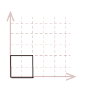
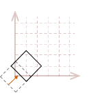
For the illustration of these transforms, we will use the two-dimensional unit-square shown below. However, I will demonstrate the math and algorithms for three dimensions.
| \( \eqalign{ pt_{1} &= (\matrix{0 & 0})\\ pt_{2} &= (\matrix{1 & 0})\\ pt_{3} &= (\matrix{1 & 1})\\ pt_{4} &= (\matrix{0 & 1})\\ }\) |
|
Translate
Translating a point in 3D space is as simple as adding the desired offset for the coordinate of each corresponding axes.
\( V_{translate}=V+D \)
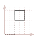
For instance, to move our sample unit cube from the origin by \(x=2\) and \(y=3\), we simply add \(2\) to the x-component for every point in the square, and \(3\) to every y-component.
| \( \eqalign{ pt_{1D} &= pt_1 + [\matrix{2 & 3}] \\ pt_{2D} &= pt_2 + [\matrix{2 & 3}] \\ pt_{3D} &= pt_3 + [\matrix{2 & 3}] \\ pt_{4D} &= pt_4 + [\matrix{2 & 3}] \\ }\) |
|
There is a better way, though.
That will have to wait until after I demonstrate the other two manipulation methods.
Identity Matrix
The first thing that we need to become familiar with is the identity matrix. The identity matrix has ones set along the diagonal with all of the other elements set to zero. Here is the identity matrix for a \(3 \times 3\) matrix.
\( \left\lbrack \matrix{1 & 0 & 0\cr 0 & 1 & 0\cr 0 & 0 & 1} \right\rbrack\)
When any valid input matrix is multiplied with the identity matrix, the result will be the unchanged input matrix. Only square matrices can identity matrices. However, non-square matrices can be used for multiplication with the identity matrix if they have compatible dimensions.
For example:
\( \left\lbrack \matrix{a & b & c \\ d & e & f \\ g & h & i} \right\rbrack \left\lbrack \matrix{1 & 0 & 0\cr 0 & 1 & 0\cr 0 & 0 & 1} \right\rbrack = \left\lbrack \matrix{a & b & c \\ d & e & f \\ g & h & i} \right\rbrack \)
\( \left\lbrack \matrix{7 & 6 & 5} \right\rbrack \left\lbrack \matrix{1 & 0 & 0\cr 0 & 1 & 0\cr 0 & 0 & 1} \right\rbrack = \left\lbrack \matrix{7 & 6 & 5} \right\rbrack \)
\( \left\lbrack \matrix{1 & 0 & 0\cr 0 & 1 & 0\cr 0 & 0 & 1} \right\rbrack \left\lbrack \matrix{7 \\ 6 \\ 5} \right\rbrack = \left\lbrack \matrix{7 \\ 6 \\ 5} \right\rbrack \)
We will use the identity matrix as the basis of our transformations.
Scale
It is possible to independently scale geometry along each of the standard axes. We first start with a \(2 \times 2\) identity matrix for our two-dimensional unit square:
\( \left\lbrack \matrix{1 & 0 \\ 0 & 1} \right\rbrack\)
As we demonstrated with the identity matrix, if we multiply any valid input matrix with the identity matrix, the output will be the same as the input matrix. This is similar to multiplying by \(1\) with scalar numbers.
\( V_{scale}=VS \)
Based upon the rules for matrix multiplication, notice how there is a one-to-one correspondence between each row/column in the identity matrix and for each component in our point..
\(\ \matrix{\phantom{x} & \matrix{x & y} \\ \phantom{x} & \phantom{x} \\ \matrix{x \\ y} & \left\lbrack \matrix{1 & 0 \\ 0 & 1} \right\rbrack } \)
We can create a linear transformation to scale point, by simply multiplying the \(1\) in the identity matrix, with the desired scale factor for each standard axis. For example, let's make our unit-square twice as large along the \(x-axis\) and half as large along the \(y-axis\):
\(\ S= \left\lbrack \matrix{2 & 0 \\ 0 & 0.5} \right\rbrack \)
This is the result, after we multiply each point in our square with this transformation matrix; I have also broken out the mathematic calculations for one of the points, \(pt_3(1, 1)\):
| \( \eqalign{ pt_{3}S &= \\ &= [\matrix{1 & 1}] \left\lbrack\matrix{2 & 0 \\ 0 & 0.5} \right\rbrack\\ &= [\matrix{(1 \cdot 2 + 1 \cdot 0) & (1 \cdot 0 + 1 \cdot 0.5)}] \\ &= [\matrix{2 & 0.5}] }\) |
|
Here is the scale transformation matrix for three dimensions:
\(S = \left\lbrack \matrix{S_x & 0 & 0 \\ 0 & S_y & 0 \\ 0 & 0 & S_z }\right\rbrack\)
Rotate
A rotation transformation can be created similarly to how we created a transformation for scale. However, this transformation is more complicated than the previous one. I am only going to present the formula, I am not going to explain the details of how it works. The matrix below will perform a counter-clockwise rotation about a pivot-point that is placed at the origin:
\(\ R= \left\lbrack \matrix{\phantom{-} \cos \Theta & \sin \Theta \\ -\sin \Theta & \cos \Theta} \right\rbrack \)
\(V'=VR\)
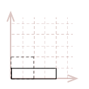
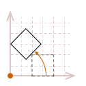
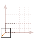
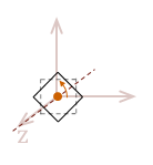
As I mentioned, the rotation transformation pivots the point about the origin. Therefore, if we attempt to rotate our unit square, the result will look like this:
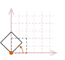
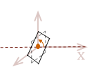
The effects become even more dramatic if the object is not located at the origin:
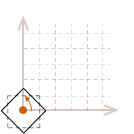
In most cases, this may not be what we would like to have happen. A simpler way to reason about rotation is to place the pivot point in the center of the object, so it appears to rotate in place.
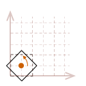
To rotate an object in place, we will need to first translate the object so the desired pivot point of the rotation is located at the origin, rotate the object, then undo the original translation to move it back to its original position.
While all of those steps must be taken in order to rotate an object about its center, there is a way to combine those three steps to create a single matrix. Then only one matrix multiplication operation will need to be performed on each point in our object. Before we get to that, let me show you how we can expand this rotation into three dimensions.
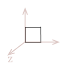
Imagine that our flat unit-square object existed in three dimensions. It is still defined to exist on the \(xy\) plane, but it has a third component added to each of its points to mark its location along the \(z-axis\). We simply need to adjust the definition of our points like this:
| \( \eqalign{ pt_{1} &= (\matrix{0 & 0 & 0})\\ pt_{2} &= (\matrix{1 & 0 & 0})\\ pt_{3} &= (\matrix{1 & 1 & 0})\\ pt_{4} &= (\matrix{0 & 1 & 0})\\ }\) |
|
So, you would be correct to surmise that in order to perform this same \(xy\) rotation about the \(z-axis\) in three dimensions, we simply need to begin with a \(3 \times 3\) identity matrix before we add the \(xy\) rotation.
| \( R_z = \left\lbrack \matrix{ \phantom{-}\cos \Theta & \sin \Theta & 0 \\ -\sin \Theta & \cos \Theta & 0 \\ 0 & 0 & 1 } \right\rbrack \) |
|
We can also adjust the rotation matrix to perform a rotation about the \(x\) and \(y\) axis, respectively:
| R_x = \( \left\lbrack \matrix{ 1 & 0 & 0 \\ 0 & \phantom{-}\cos \Theta & \sin \Theta \\ 0 & -\sin \Theta & \cos \Theta } \right\rbrack \) |
|
| \( R_y = \left\lbrack \matrix{ \cos \Theta & 0 & -\sin \Theta\\ 0 & 1 & 0 \\ \sin \Theta & 0 & \phantom{-}\cos \Theta } \right\rbrack \) |
|
Composite Transform Matrices
I mentioned that it is possible to combine a sequence of matrix transforms into a single matrix. This is highly desirable, considering that every point in an object model needs to be multiplied by the transform. What I demonstrated up to this point is how to individually create each of the transform types, translate, scale and rotate. Technically, the translate operation, \(V'=V+D\) is not a linear transformation because it is not composed within a matrix. Before we can continue, we must find a way to turn the translation operation from a matrix add to a matrix multiplication.
It turns out that we can create a translation operation that is a linear transformation by adding another row to our transformation matrix. However, a transformation matrix must be square because it starts with the identity matrix. So we must also add another column, which means we now have a \(4 \times 4\) matrix:
\(T = \left\lbrack \matrix{1 & 0 & 0 & 0\\ 0 & 1 & 0 & 0\\ 0 & 0 & 1 & 0\\ t_x & t_y & t_z & 1 }\right\rbrack\)
A general transformation matrix is in the form:
\( \left\lbrack \matrix{ a_{11} & a_{12} & a_{13} & 0\\ a_{21} & a_{22} & a_{23} & 0\\ a_{31} & a_{32} & a_{33} & 0\\ t_x & t_y & t_z & 1 }\right\rbrack\)
Where \(t_x\),\(t_y\) and \(t_z\) are the final translation offsets, and the sub-matrix \(a\) is a combination of the scale and rotate operations.
However, this matrix is not compatible with our existing point definitions because they only have three components.
Homogenous Coordinates
The final piece that we need to finalize our geometry representation and coordinate management logic is called Homogenous Coordinates. What this basically means, is that we will add one more parameter to our vector definition. We refer to this fourth component as, \(w\), and we initially set it to \(1\).
\(V(x,y,z,w) = [\matrix{x & y & z & 1}]\)
Our vector is only valid when \(w=1\). After we transform a vector, \(w\) has often changed to some other scale factor. Therefore, we must rescale our vector back to its original basis by dividing each component by \(w\). The equations below show the three-dimensional Cartesian coordinate representation of a vector, where \(w \ne 0\).
\( \eqalign{ x&= X/w \\ y&= Y/w \\ z&= Z/w }\)
Creating a Composite Transform Matrix
We now possess all of the knowledge required to compose a linear transformation sequence that is stored in a single, compact transformation matrix. So let's create the rotation sequence that we discussed earlier. We will a compose a transform that translates an object to the origin, rotates about the \(z-axis\) then translates the object back to its original position.
Each individual transform matrix is shown below in the order that it must be multiplied into the final transform.
\( T_c R_z T_o = \left\lbrack \matrix{ 1 & 0 & 0 & 0 \\ 0 & 1 & 0 & 0 \\ 0 & 0 & 1 & 0 \\ -t_x & -t_y & -t_z & 1 \\ } \right\rbrack \left\lbrack \matrix{ \phantom{-}\cos \Theta & \sin \Theta & 0 & 0 \\ -\sin \Theta & \cos \Theta & 0 & 0 \\ 0 & 0 & 1 & 0 \\ 0 & 0 & 0 & 1 \\ } \right\rbrack \left\lbrack \matrix{ 1 & 0 & 0 & 0 \\ 0 & 1 & 0 & 0 \\ 0 & 0 & 1 & 0 \\ t_x & t_y & t_z & 1 \\ } \right\rbrack \)
Here, values are selected and the result matrix is calculated:
\(t_x = 0.5, t_y = 0.5, t_z = 0.5, \Theta = 45°\)
\( \eqalign{ T_c R_z T_o &= \left\lbrack \matrix{ 1 & 0 & 0 & 0 \\ 0 & 1 & 0 & 0 \\ 0 & 0 & 1 & 0 \\ -0.5 & -0.5 & -0.5 & 1 \\ } \right\rbrack \left\lbrack \matrix{ 0.707 & 0.707 & 0 & 0 \\ -0.707 & 0.707 & 0 & 0 \\ 0 & 0 & 1 & 0 \\ 0 & 0 & 0 & 1 \\ } \right\rbrack \left\lbrack \matrix{ 1 & 0 & 0 & 0 \\ 0 & 1 & 0 & 0 \\ 0 & 0 & 1 & 0 \\ 0.5 & 0.5 & 0.5 & 1 \\ } \right\rbrack \\ \\ &=\left\lbrack \matrix{ \phantom{-}0.707 & 0.707 & 0 & 0 \\ -0.707 & 0.707 & 0 & 0 \\ 0 & 0 & 1 & 0 \\ 0.5 & -0.207 & 0 & 1 \\ } \right\rbrack }\)
It is possible to derive the final composite matrix by using algebraic manipulation to multiply the transforms with the unevaluated variables. The matrix below is the simplified definition for \(T_c R_z T_o\) from above:
\( T_c R_z T_o = \left\lbrack \matrix{ \phantom{-}\cos \Theta & \sin \Theta & 0 & 0 \\ -\sin \Theta & \cos \Theta & 0 & 0 \\ 0 & 0 & 1 & 0 \\ (-t_x \cos \Theta + t_y \sin \Theta + t_x) & (-t_x \sin \Theta - t_y \cos \Theta + t_y) & 0 & 1 \\ } \right\rbrack\)
Projection Transformation
The last thing to do, is to convert our 3D model into an image. We have three-dimensional coordinates, that must be mapped to a two-dimensional surface. To do this, we will project a view of our world-space onto a flat two-dimensional screen. This is known as the "projection transformation" or "projection matrix".
Coordinate Systems
It may be already be apparent, but if not I will state it anyway; a linear transformation is a mapping between two coordinate systems. Whether we translate, scale or rotate we are simply changing the location and orientation of the origin. We have actually used the origin as our frame of reference, so our transformations appear to be moving our geometric objects. This is a valid statement, because the frame of reference determines many things.
We need a frame of reference that can be used as the eye or camera. We call this frame of reference the view space and the eye is located at the view-point. In fact, up to this point we have also used two other vector-spaces, local space (also called model space and world space. To be able to create our projection transformation, we need to introduce one last coordinate space called screen space. Screen space is a 2D coordinate system defined by the \(uv-plane\), and it maps directly to the display image or screen.
The diagram below depicts all four of these different coordinate spaces:
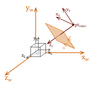
The important concept to understand, is that all of these coordinate systems are relatively positioned, scaled, and oriented to each other. We construct our transforms to move between these coordinate spaces. To render a view of the scene, we need to construct a transform to go from world space to view space.
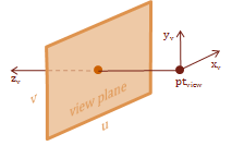
View Space
The view space is the frame of reference for the eye. Basically, our view of the scene. This coordinate space allows us to transform the world coordinates to a position relative to our view point. This makes it possible for us to create a projection of this visible scene onto our view plane.
We need a point and two vectors to define the location and orientation of the view space. The method I demonstrate here is called the "eye, at, up" method. This is because we specify a point to be the location of the eye, a vector from the eye to the focal-point, at, and a vector that indicates which direction is up. I like this method because I think it is an intuitive model for visualizing where your view-point is located, how it is oriented, and what you are looking at.
Right or Left Handed?
The view space is a left-handed coordinate system, which differs from the right-handed coordinate systems that we have used up to this point. In math and physics, right-handed systems are the norm. This places the \(y-axis\) up, and the \(x-axis\) pointing to the right (same as the classic 2D Cartesian grid), and the resulting \(z-axis\) will point toward you. For a left-handed space, the positive \(z-axis\) points into the paper. This makes things very convenient in computer graphics, because \(z\) is typically used to measure and indicate depth.
You can tell which type of coordinate system that you have created by taking your open palm and pointing it perpendicularly to the \(x-axis\), and your palm facing the \(y-axis\). The positive \(z-axis\) will point in the direction of your thumb, based upon the direction your coordinate space is oriented.
Let's define a simple view space transformation.
\( \eqalign{ eye&= [\matrix{2 & 3 & 3}] \\ at&= [\matrix{0 & 0 & 0}] \\ up&= [\matrix{0 & 1 & 0}] }\)
Simple Indeed.
From this, we can create a view located at \([\matrix{2 & 3 & 3}]\) that is looking at the origin and is oriented vertically (no tilt to either side). We start by using the vector operations, which I demonstrated in my previous post, to define vectors for each of the three coordinate axes.
\( \eqalign{ z_{axis}&= \| at-eye \| \\ &= \| [\matrix{-2 & -3 & -3}] \| \\ &= [\matrix{-0.4264 & -0.6396 & -0.6396}] \\ \\ x_{axis}&= \| up \times z_{axis} \| \\ &=\| [\matrix{-3 & 0 & 2}] \|\\ &=[\matrix{-0.8321 & 0 & 0.5547}]\\ \\ y_{axis}&= \| z_{axis} \times x_{axis} \| \\ &= [\matrix{-0.3547 & -0.7687 & -0.5322}] }\)
We now take these three vectors, and plug them into this composite matrix that is designed to transform world space to a new coordinate space defined by axis-aligned unit vectors.
\( \eqalign { T_{view}&=\left\lbrack \matrix{ x_{x_{axis}} & x_{y_{axis}} & x_{z_{axis}} & 0 \\ y_{x_{axis}} & y_{y_{axis}} & y_{z_{axis}} & 0 \\ z_{x_{axis}} & z_{y_{axis}} & z_{z_{axis}} & 0 \\ -(x_{axis} \cdot eye) & -(y_{axis} \cdot eye) & -(z_{axis} \cdot eye) & 1 \\ } \right\rbrack \\ \\ &=\left\lbrack \matrix{ -0.8321 & -0.3547 & -0.4264 & 0 \\ 0 & -0.7687 & -0.6396 & 0 \\ -0.5547 & -0.5322 & -0.6396 & 0 \\ 3.3283 & 4.6121 & 4.6904 & 1 \\ } \right\rbrack }\)
Gaining Perspective
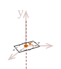
The final step is to project what we can see from the \(eye\) in our view space, onto the view-plane. As I mentioned previous, the view-plane is commonly referred to as the \(uv-plane\). The \(uv\) coordinate-system refers to the 2D mapping on the \(uv-plane\). The projection mapping that I demonstrate here places the \(uv-plane\) some distance \(d\) from the \(eye\), so that the view-space \(z-axis\) is parallel with the plane's normal.
The \(eye\) is commonly referred to by another name for the context of the projection transform, it is called the center of projection. That is because this final step, basically, projects the intersection of a projected vector onto the \(uv-plane\). The projected vector originates at the center of projection and points to each point in the view-space.
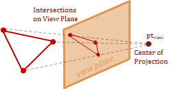
The cues that let us perceive perspective with stereo-scopic vision is called, fore-shortening. This effect is caused by objects appearing much smaller as they are further from our vantage-point. Therefore, we can recreate the foreshortening in our image by scaling the \(xy\) values based on their \(z\)-coordinate. Basically, the farther away an object is placed from the center of projection, the smaller it will appear.
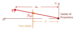
The diagram above shows a side view of the \(y\) and \(z\) axes, and is parallel with the \(x-axis\). Notice the have similar triangles that are created by the view plane. The smaller triangle on the bottom is the distance \(d\), which is the distance from the center of projection to the view plane. The larger triangle on the top extends from the point \(Pv\) to the \(y-axis\), this distance is the \(z\)-component value for the point \(Pv\). Using the property of similar triangles we now have a geometric relationship that allows us to scale the location of the point for the view plane intersection.
|
\(\frac{x_s}d = \frac{x_v}{z_v}\) |
\(\frac{y_s}d = \frac{y_v}{z_v}\) |
|
\(x_s = \frac{x_v}{z_v/d}\) |
\(y_s = \frac{y_v}{z_v/d}\) |
With this, we can define a perspective-based projection transform:
\( T_{project}=\left\lbrack \matrix{ 1 & 0 & 0 & 0 \\ 0 & 1 & 0 & 0 \\ 0 & 0 & 1 & 1/d \\ 0 & 0 & 0 & 0} \right\rbrack \)
This is now where the homogenizing component \(w\) returns. This transform will have the affect of scaling the \(w\) component to create:
\( \eqalign{ X&= x_v \\ Y&= y_v \\ Z&= z_v \\ w&= z_v/d }\)
Which is why we need to access these values as shown below after the following transform is used:
\( \eqalign{ [\matrix{X & Y & Z & w}] &= [\matrix{x_v & y_v & z_v & 1}] T_{project}\\ \\ x_v&= X/w \\ y_v&= Y/w \\ z_v&= Z/w }\)
Scale the Image Plane
Here is one last piece of information that I think you will appreciate. The projection transform above defines a \(uv\) coordinate system that is \(1 \times 1\). Therefore, if you make the following adjustment, you will scale the unit-plane to match the size of your final image in pixels:
\( T_{project}=\left\lbrack \matrix{ width & 0 & 0 & 0 \\ 0 & height & 0 & 0 \\ 0 & 0 & 1 & 1/d \\ 0 & 0 & 0 & 0} \right\rbrack \)
Summary
We made it! With a little bit of knowledge from both Linear Algebra and Trigonometry, we have been able to construct and manipulate geometric models in 3D space, concatenate transform matrices into compact and efficient transformation definitions, and finally create a projection transform to create a two-dimensional image from a three-dimensional definition.
As you can probably guess, this is only the beginning. There is so much more to explore in the creation of computer graphics. Some of the more interesting topics that generally follow after the 3D projection is created are:
- Shading Models: Flat, Gouraud and Phong.
- Shadows
- Reflections
- Transparency and Refraction
- Textures
- Bump-mapping ...
The list goes on and on. I imagine that I will continue to write on this topic and address polygon fill algorithms and the basic shading models. However, I think things will be more interesting if I have code to demonstrate and possibly an interactive viewer for the browser. I have a few demonstration programs written in C++ for Windows, but I would prefer to create something that is a bit more portable.
Once I decide how I want to proceed I will return to this topic. However, if enough people express interest, I wouldn't mind continuing forward demonstrating with C++ Windows programs. Let me know what you think.
References
Watt, Alan, "Three-dimensional geometry in computer graphics," in 3D Computer Graphics, Harlow, England: Addison-Wesley, 1993
Foley, James, D., et al., "Geometrical Transformations," in Computer Graphics: Principles and Practice, 2nd ed. in C, Reading: Addison-Wesley, 1996

Recent Comments