| « 3D Projection and Matrix Transforms | Introduction to the Math of Computer Graphics » |
I previously introduced how to perform the basic matrix operations commonly used in 3D computer graphics. However, we haven’t yet reached anything that resembles graphics. I now introduce the concepts of geometry as it’s related to computer graphics. I intend to provide you with the remaining foundation necessary to be able to mathematically visualize the concepts at work. Unfortunately, we will still not be able to reach the "computer graphics" stage with this post; that must wait until the next entry.
This post covers a basic form of a polygonal mesh to represent models, points and Euclidean vectors. With the previous entry and this one, we will have all of the background necessary for me to cover matrix transforms in the next post. Specifically the 3D projection transform, which provides the illusion of perspective. This will be everything that we need to create a wireframe viewer. For now, let's focus on the topics of this post.
Modeling the Geometry
We will use models composed of a mesh of polygons. All of the polygons will be defined as triangles. It is important to consistently define the points of each triangle either clockwise or counter-clockwise. This is because the definition order affects the direction a surface faces. If a single model mixes the order of point definitions, your rendering will have missing polygons.
The order of point definition for the triangle can be ignored if a surface normal is provided for each polygon. However, to keep things simple, I will only be demonstrating with basic models that are built from an index array structure. This data structure contains two arrays. The first array is a list of all of the vertices (points) in the model. The second array contains a three-element structure with the index of the point that can be found in the first array. I define all of my triangles counter-clockwise while looking at the front of the surface.
Generally, your models should be defined at or near the origin. The rotation transformation that we will explore in the next post requires a pivot point, which is defined at the origin. Model geometries defined near the origin are also easier to work with when building models from smaller components and using instancing to create multiple copies of a single model.
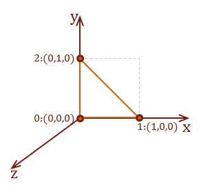
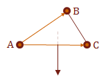
Here is a definition for a single triangle starting at the origin and adjacent to the Y plane. The final corner decreases for Y as it moves diagonally along the XZ plane:
|
|
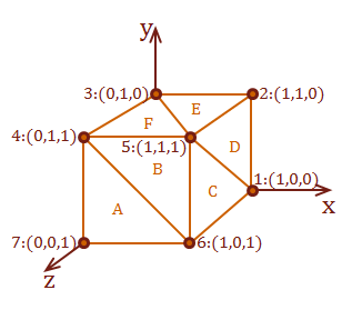
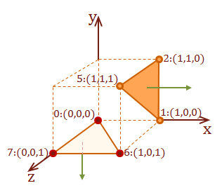
This definition represents a unit cube starting at the origin. A cube has 8 corners to hold six square-faces. It requires two triangles to represent each square. Therefore, there are 8 points used to define 12 triangles:
|
|
Vectors
Recall from my previous post that a vector is a special type of matrix, in which there is only a single row or column. You may be aware of a different definition for the term "vector"; something like
NOUN
A quantity having direction as well as magnitude, especially determining the position of one point in space relative to another.
Oxford Dictionary
From this point forward, when I use the term "vector", I mean a Euclidean vector. We will even use single-row and single-column matrices to represent these vectors; we’re just going to refer to those structures as matrices to minimize the confusion.
Notational Convention
It is most common to see vectors represented as single-row matrices, as opposed to the standard mathematical notation which uses column matrices to represent vectors. It is important to remember this difference in notation based on what type of reference you are following.
The reason for this difference, is the row-form makes composing the transformation matrix more natural as the operations are performed left-to-right. I discuss the transformation matrix in the next entry. As you will see, properly constructing transformation matrices is crucial to achieve the expected results, and anything that we can do to simplify this sometimes complex topic, will improve our chances of success.
Representation
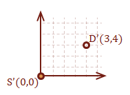
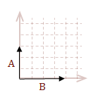
As the definition indicates, a vector has a direction and magnitude. There is a lot of freedom in that definition for representation, because it is like saying "I don’t know where I am, but I know which direction I am heading and how far I can go." Therefore, if we think of our vector as starting at the origin of a Cartesian grid, we could then represent a vector as a single point.
This is because starting from the origin, the direction of the vector is towards the point. The magnitude can be calculated by using Pythagoras' Theorem to calculate the distance between two points. All of this information can be encoded in a compact, single-row matrix. As the definition indicates, we derive a vector from two points, by subtracting one point from the other using inverse of matrix addition.
This will give us the direction to the destination point, relative to the starting point. The subtraction effectively acts as a translation of the vectors starting point to the origin.
For these first few vector examples, I am going to use 2D vectors. Because they are simpler to demonstrate and diagram, and the only difference to moving to 3D vectors is an extra field has been added.
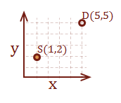
Here is a simple example with two points (2, 1) and (5, 5). The first step is to encode them in a matrix:
\( {\bf S} = \left\lbrack \matrix{2 & 1} \right\rbrack, {\bf D} = \left\lbrack \matrix{5 & 5} \right\rbrack \)
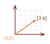
Let’s create two vectors, one that determines how to get to point D starting from S, and one to get to point S starting from D. The first step is to subtract the starting point from the destination point. Notice that if we were to subtract the starting point from itself, the result is the origin, (0, 0).
\( \eqalign{ \overrightarrow{SD} &= [ \matrix{5 & 5} ] - [ \matrix{2 & 1} ] \cr &= [ \matrix{3 & 4} ] } \)
\( \eqalign{ \overrightarrow{DS} &= [ \matrix{2 & 1} ] - [ \matrix{5 & 5} ] \cr &= [ \matrix{-3 & -4} ] } \)
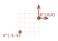
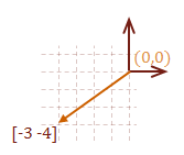
Notice that the only difference between the two vectors is the direction. The magnitude of each vector is the same, as expected. Here is how to calculate the magnitude of a vector:
Given:
\( \eqalign{ v &= \matrix{ [a_1 & a_2 & \ldots & a_n]} \cr |v| &= \sqrt{\rm (a_1^2 + a_2^2 + \ldots + a_n^2)} } \)
Operations
I covered scalar multiplication and matrix addition in my previous post. However, I wanted to briefly revisit the topic to demonstrate one way to think about vectors, which may help you develop a better intuition for the math. For the coordinate systems that we are working with, vectors are straight lines.
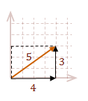
When you add two or more vectors together, you can think of them as moving the tail of each successive vector to the head of the previous vector. Then add the corresponding components.
\( \eqalign{ v &= A+B \cr |v| &= \sqrt{\rm 3^2 + 4^2} \cr &= 5 }\)
Regardless of the orientation of the vector, it can be decomposed into its individual contributions per axis. In our model for the vector, the contribution for each axis is the raw value defined in our matrix.
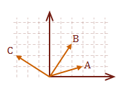
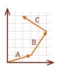
\( v = A+B+C \)
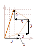
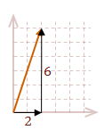
\( \eqalign{ |v| &= \sqrt{\rm (3+2-3)^2 + (1+3+2)^2} \cr &= \sqrt{\rm 2^2 + 6^2} \cr &= 2 \sqrt{\rm 10} }\)
Unit Vector
We can normalize a vector to create unit vector, which is a vector that has a length of 1. The concept of the unit vector is introduced to reduce a vector to simply indicate its direction. This type of vector can now be used as a unit of measure to which other vectors can be compared. This also simplifies the task of deriving other important information when necessary.
To normalize a vector, divide the vector by its magnitude. In terms of the matrix operations that we have discussed, this is simply scalar multiplication of the vector with the inverse of its magnitude.
\( u = \cfrac{v}{ |v| } \)
\(u\) now contains the information for the direction of \(v\). With algebraic manipulation we can also have:
\( v = u |v| \)
This basically says the vector \(v\) is equal to the unit vector that has the direction of \(u\) multiplied by the magnitude of \(v\).
Dot Product
The dot product is used for detecting visibility and shading of a surface. The dot product operation is shown below:
\( \eqalign{ w &= u \cdot v \cr &= u_1 v_1 + u_2 v_2 + \cdots + u_n v_n }\)
This formula may look familiar. That is because this is a special case in matrix multiplication called the inner product, which looks like this (remember, we are representing vectors as a row matrix):
\( \eqalign{ u \cdot v &= u v^T \cr &= \matrix {[u_1 & u_2 & \cdots & u_n]} \left\lbrack \matrix{v_1 \\ v_2 \\ \vdots \\ v_n } \right\rbrack }\)
We will use the dot product on two unit vectors to help us determine the angle between these vectors; that’s right, angle. We can do this because of the cosine rule from Trigonometry. The equation that we can use is as follows:
\( \cos \Theta = \cfrac{u \cdot v} {|u||v|} \)
To convert this to the raw angle, \(\Theta\), you can use the inverse function of cosine, arccos(\( \Theta \)). In C and C++ the name of the function is acos().
\( \cos {\arccos \Theta} = \Theta \)
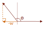
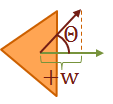
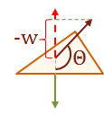
So what is actually occurring when we calculate the dot product that allows us to get an angle?
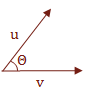
We are essentially calculating the projection of u onto v. This gives us enough information to manipulate the Trigonometric properties to derive \( \Theta \).

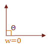
I would like to make one final note regarding the dot product. Many times it is only necessary to know the sign of the angle between two vectors. The following table shows the relationship between the dot product of two vectors and the value of the angle, \( \Theta \), which is in the range \( 0° \text{ to } 180° \). If you like radians, that is \( 0 \text{ to } \pi \).
\( w = u \cdot v = f(u,w) \)
\( f(u,w) = \cases{ w \gt 0 & \text { if } \Theta \lt 90° \cr w = 0 & \text { if } \Theta = 90° \cr w \lt 0 & \text { if } \Theta \gt 90° }\)
Cross Product
The cross product is used to calculate a vector that is perpendicular to a surface. The name for this vector is the surface normal. The surface normal indicates which direction the surface is facing. Therefore, it is used quite extensively for shading and visibility as well.
We have reached the point where we need to start using examples and diagrams with three dimensions. We will use the three points that define our triangular surface to create two vectors. Remember, it is important to use consistent definitions when creating models.
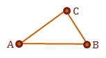
The first step is to calculate our planar vectors. What does that mean? We want to create two vectors that are coplanar (on the same plane), so that we may use them to calculate the surface normal. All that we need to be able to do this are three points that are non-collinear, and we have this with each triangle definition in our polygonal mesh model.
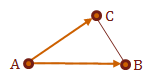
If we have defined a triangle \(\triangle ABC\), we will define two vectors, \(u = \overrightarrow{AB}\) and \(v = \overrightarrow{AC}\).
If we consistently defined the triangle surfaces in our model, we should now be able to take the cross product of \(u \times v\) to receive the surface normal, \(N_p\), of \(\triangle ABC\). Again, the normal vector is perpendicular to its surface.
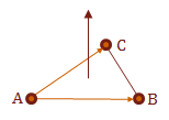
In practice, this tells us which direction the surface is facing. We would combine this with the dot product to help us determine if are interested in this surface for the current view.
So how do you calculate the cross product?
Here is what you need to know in order to calculate the surface normal vector:
\(\eqalign { N_p &= u \times v \cr &= [\matrix{(u_2v_3 – u_3v_2) & (u_3v_1 – u_1v_3) & (u_1v_2 – u_2v_1)}] }\)
To help you remember how to perform the calculation, I have re-written it in parts, and used \(x\), \(y\), and \(z\) rather than the index values.
\(\eqalign { x &= u_yv_z – u_zv_y \cr y &= u_zv_x – u_xv_z \cr z &= u_xv_y – u_yv_x }\)
Let's work through an example to demonstrate the cross product. We will use surface A from our axis-aligned cube model that we constructed at the beginning of this post. Surface A is defined completely within the XY plane. How do we know this? Because all of the points have the same \(z\)-coordinate value of 1. Therefore, we should expect that our calculation for \(N_p\) of surface A will be an \(z\) axis-aligned vector pointing in the positive direction.
Step 1: Calculate our surface description vectors \(u\) and \(v\):
\( Surface_A = pt_7: (0,0,1), pt_6: (1,0,1), \text{ and } pt_4: (0,1,1) \)
|
\( \eqalign { u &= pt_6 - pt_7 \cr &= [\matrix{1 & 0 & 1}] - [\matrix{0 & 0 & 1}] \cr &=[\matrix{\color{red}{1} & \color{green}{0} & \color{blue}{0}}] }\) |
\( \eqalign { v &= pt_4 - pt_7 \cr &= [\matrix{0 & 1 & 1}] - [\matrix{0 & 0 & 1}] \cr &=[\matrix{\color{red}{0} & \color{green}{1} & \color{blue}{0}}] }\) |
Step 2: Calculate \(u \times v\):
\(N_p = [ \matrix{x & y & z} ]\text{, where:}\)
|
\( \eqalign { x &= \color{green}{u_y}\color{blue}{v_z} – \color{blue}{u_z}\color{green}{v_y} \cr &= \color{green}{0} \cdot \color{blue}{0} - \color{blue}{0} \cdot \color{green}{1} \cr &= 0 }\) |
\( \eqalign { y &= \color{blue}{u_z}\color{red}{v_x} – \color{red}{u_x}\color{blue}{v_z} \cr &= \color{blue}{0} \cdot \color{red}{0} - \color{red}{1} \cdot \color{blue}{0} \cr &= 0 }\) |
\( \eqalign { z &= \color{red}{u_x}\color{green}{v_y} – \color{green}{u_y}\color{red}{v_x} \cr &= \color{red}{1} \cdot \color{green}{1} - \color{green}{0} \cdot \color{red}{0} \cr &= 1 }\) |
\(N_p = [ \matrix{0 & 0 & 1} ]\)
This is a \(z\) axis-aligned vector pointing in the positive direction, which is what we expected to receive.
Notation Formality
If you look at other resources to learn more about the cross product, it is actually defined as a sum in terms of three axis-aligned vectors \(i\), \(j\), and \(k\), which then must be multiplied by the vectors \(i=[\matrix{1&0&0}]\), \(j=[\matrix{0&1&0}]\), and \(k=[\matrix{0&0&1}]\) to get the final vector. The difference between what I presented and the form with the standard vectors, \(i\), \(j\), and \(k\), is I omitted a step by placing the result calculations directly in a new vector. I wanted you to be aware of this discrepancy between what I have demonstrated and what is typically taught in the classroom.
Apply What We Have Learned
We have discovered quite a few concepts between the two posts that I have written regarding the basic math and geometry involved with computer graphics. Let's apply this knowledge and solve a useful problem. Detecting if a surface is visible from a specific point-of-view is a fundamental problem that is used extensively in this domain. Since we have all of the tools necessary to solve this, let's run through two examples.
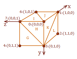
For the following examples we will specify the view-point as \(pt_{eye} = [\matrix{3 & 2 & 3}]:\)
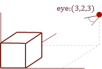
Also, refer to this diagram for the surfaces that we will test for visibility from the view-point. The side surface is surface \(D\) from the cube model, and the hidden surface is the bottom-facing surface \(J\).
Detect a visible surface
Step 1: Calculate our surface description vectors \(u\) and \(v\):
\( \eqalign{ Surface_D: &pt_5: (1,1,1), \cr &pt_1: (1,0,0), \cr &pt_2: (1,1,0) } \)
|
\( \eqalign { u &= pt_1 - pt_5 \cr &= [\matrix{1 & 0 & 0}] - [\matrix{1 & 1 & 1}] \cr &=[\matrix{0 & -1 & -1}] }\) |
\( \eqalign { v &= pt_2 - pt_5 \cr &= [\matrix{1 & 1 & 0}] - [\matrix{1 & 1 & 1}] \cr &=[\matrix{0 & 0 & -1}] }\) |
Step 2: Calculate \(u \times v\):
\(N_{pD} = [ \matrix{x & y & z} ]\text{, where:}\)
|
\( \eqalign { x &= -1 \cdot (-1) - (-1) \cdot 0 \cr &= 1 }\) |
\( \eqalign { y &= -1 \cdot 0 - (-1) \cdot 0 \cr &= 0 }\) |
\( \eqalign { z &= 0 \cdot 0 - (-1) \cdot 0 \cr &= 0 }\) |
\(N_pD = [ \matrix{1 & 0 & 0} ]\)
Step 3: Calculate vector to the eye:
To calculate a vector to the eye, we need to select a point on the target surface and create a vector to the eye. For this example, we will select \(pt_5\)
\( \eqalign{ \overrightarrow{view_D} &= pt_{eye} - pt_5\cr &= [ \matrix{3 & 2 & 3} ] - [ \matrix{1 & 1 & 1} ]\cr &= [ \matrix{2 & 1 & 2} ] }\)
Step 4: Normalize the view-vector:
Before we can use this vector in a dot product, we must normalize the vector:
\( \eqalign{ |eye_D| &= \sqrt{\rm 2^2 + 1^2 + 2^2} \cr &= \sqrt{\rm 4 + 1 + 4} \cr &= \sqrt{\rm 9} \cr &= 3 \cr \cr eye_u &= \cfrac{eye_D}{|eye_D|} \cr &= \cfrac{1}3 [\matrix{2 & 1 & 2}] \cr &= \left\lbrack\matrix{\cfrac{2}3 & \cfrac{1}3 & \cfrac{2}3} \right\rbrack }\)
Step 5: Calculate the dot product of the view-vector and surface normal:
\( \eqalign{ w &= eye_{u} \cdot N_{pD} \cr &= \cfrac{2}3 \cdot 1 + \cfrac{1}3 \cdot 0 + \cfrac{2}3 \cdot 0 \cr &= \cfrac{2}3 }\)
Step 6: Test for visibility:
|
\(w \gt 0\), therefore \(Surface_D\) is visible. |
|
Detect a surface that is not visible
Step 1: Calculate our surface description vectors \(u\) and \(v\):
\( \eqalign{ Surface_J: &pt_6: (1,1,1), \cr &pt_0: (0,0,0), \cr &pt_1: (1,0,0) } \)
|
\( \eqalign { u &= pt_0 - pt_6 \cr &= [\matrix{0 & 0 & 0}] - [\matrix{1 & 0 & 1}] \cr &=[\matrix{-1 & 0 & -1}] }\) |
\( \eqalign { v &= pt_1 - pt_6 \cr &= [\matrix{1 & 0 & 0}] - [\matrix{1 & 0 & 1}] \cr &=[\matrix{0 & 0 & -1}] }\) |
Step 2: Calculate \(u \times v\):
\(N_{pJ} = [ \matrix{x & y & z} ]\text{, where:}\)
|
\( \eqalign { x &= 0 \cdot (-1) - (-1) \cdot 0 \cr &= 0 }\) |
\( \eqalign { y &= -1 \cdot 0 - (-1) \cdot (-1) \cr &= -1 }\) |
\( \eqalign { z &= (-1) \cdot 0 - 0 \cdot 0 \cr &= 0 }\) |
\(N_pJ = [ \matrix{0 & -1 & 0} ]\)
Step 3: Calculate vector to the eye:
For this example, we will select \(pt_6\)
\( \eqalign{ \overrightarrow{view_J} &= pt_{eye} - pt_6\cr &= [ \matrix{3 & 2 & 3} ] - [ \matrix{1 & 0 & 1} ]\cr &= [ \matrix{2 & 2 & 2} ] }\)
Step 4: Normalize the view-vector:
Before we can use this vector in a dot product, we must normalize the vector:
\( \eqalign{ |eye_J| &= \sqrt{\rm 2^2 + 2^2 + 2^2} \cr &= \sqrt{\rm 4 + 4 + 4} \cr &= \sqrt{\rm 12} \cr &= 2 \sqrt{\rm 3} \cr \cr eye_u &= \cfrac{eye_J}{|eye_J|} \cr &= \cfrac{1}{2 \sqrt 3} [\matrix{2 & 2 & 2}] \cr &= \left\lbrack\matrix{\cfrac{1}{\sqrt 3} & \cfrac{1}{\sqrt 3} & \cfrac{1}{\sqrt 3}} \right\rbrack }\)
Step 5: Calculate the dot product of the view-vector and surface normal:
\( \eqalign{ w &= eye_{u} \cdot N_{pJ} \cr &= \cfrac{1}{\sqrt 3} \cdot 0 + \cfrac{1}{\sqrt 3} \cdot (-1) + \cfrac{1}{\sqrt 3} \cdot 0 \cr &= -\cfrac{1}{\sqrt 3} }\)
Step 6: Test for visibility:
|
\(w \lt 0\), therefore \(Surface_J\) is not visible. |
|
What has this example demonstrated?
Surprisingly, this basic task demonstrates every concept that we have learned from the two posts up to this point:
- Matrix Addition: Euclidean vector creation
- Scalar Multiplication: Unit vector calculation, multiplying by \(1 / |v| \).
- Matrix Multiplication: Dot Product calculation, square-matrix multiplication will be used in the next post.
- Geometric Model Representation: The triangle surface representation provided the points for our calculations.
- Euclidean Vector: Calculation of each surfaces planar vectors, as well as the view vector.
- Cross Product: Calculation of the surface normal, \(N_p\).
- Unit Vector: Preparation of vectors for dot product calculation.
- Dot Product: Used the sign from this calculation to test for visibility of a surface.
Summary
Math can be difficult sometimes, especially with all of the foreign notation. However, with a bit of practice the notation will soon become second nature and many calculations can be performed in your head, similar to basic arithmetic with integers. While many graphics APIs hide these calculations from you, don't be fooled because they still exist and must be performed to display the three-dimensional images on your screen. By understanding the basic concepts that I have already demonstrated, you will be able to better troubleshoot your graphics programs when something wrong occurs. Even if you rely solely on a graphics library to abstract the complex mathematics.
There is only one more entry to go, and we will have enough basic knowledge of linear algebra, Euclidean geometry, and computer displays to be able to create, manipulate and display 3D models programmatically. The next entry discusses how to translate, scale and rotate geometric models. It also describes what must occur to create the illusion of a three-dimensional image on a two-dimensional display with the projection transform.
References
Watt, Alan, "Three-dimensional geometry in computer graphics," in 3D Computer Graphics, Harlow, England: Addison-Wesley, 1993

Recent Comments